R Package ‘nnet’ 详解

起因：在一次构建模型的过程中发现，用caret Package中的nnet method比使用nnet Package中的nnet效果更好（合作者的说明，准确性待验证），因此来更深层次的学习nnet与catet Package中nnet的实现原理

获取文档

从CRAN Packages By Name网站中获取到nnet与caret的文档。
nnet相对简单，而caret极其复杂，还需要用到它的学习手册。

文档内容

nnet 包中主要有如下几部分内容

• class.ind
• multinom
• nnet
• nnetHess
• predict.nnet
• which.is.max

为解决问题，目前只需考虑学习nnet即可，这也是大部分人用所需要了解的部分。但为了契合本文标题，其他各部分内容于后续补充。

下图为nnet方法及其用法说明

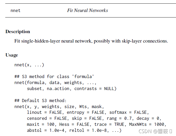
nnet介绍

nnet是一个只有单一隐藏层的神经网络，也可以跳过这个隐藏层连接（通过设置size为0，见后面参数介绍），因此从其网络结构来看，其效果必然有限，无法出色解决十分复杂的问题。

使用方法

一共有两种使用方法如下。讲解顺序如下：先举运行实例，再对其中的参数进行说明

使用类formula

## S3 method for class 'formula'
nnet(formula, data, weights, ..., subset, na.action, contrasts = NULL)

正常理解X、Y方法

## Default S3 method
nnet(x, y, weights, )

运行实例如下

rm(list = ls())
library(nnet)
# use the iris3 dataset as an example （a built-in dataset)
dim(iris)	# output: [1] 50 4 3

## Default S3 method
# construct the factor X and targets Y
ir <- rbind(iris3[,,1],iris3[,,2],iris3[,,3])
targets <- class.ind( c(rep("s", 50), rep("c", 50), rep("v", 50)) )
# sampling, half of each kind
samp <- c(sample(1:50,25), sample(51:100,25), sample(101:150,25))
# built and train ANN model
ir1 <- nnet(ir[samp,], targets[samp,], size = 2, rang = 0.1, decay = 5e-4, maxit = 200)
# check the prediction of this model
test.cl <- function(true, pred) {
	true <- max.col(true)
	cres <- max.col(pred)
	table(true, cres)
}
test.cl(targets[-samp,], predict(ir1, ir[-samp,]))
# check the parameters of this model
summary(ir1)

## or
# construct the dataset
ird <- data.frame(rbind(iris3[,,1], iris3[,,2], iris3[,,3]), species = factor(c(rep("s",50), rep("c", 50), rep("v", 50))))
# built and train ANN model
ir.nn2 <- nnet(species ~ ., data = ird, subset = samp, size = 2, rang = 0.1, decay = 5e-4, maxit = 200)
# check the prediction of this model
table(ird$species[-samp], predict(ir.nn2, ird[-samp,], type = "class"))
# check the parameters of this model
summary(ir.nn2)

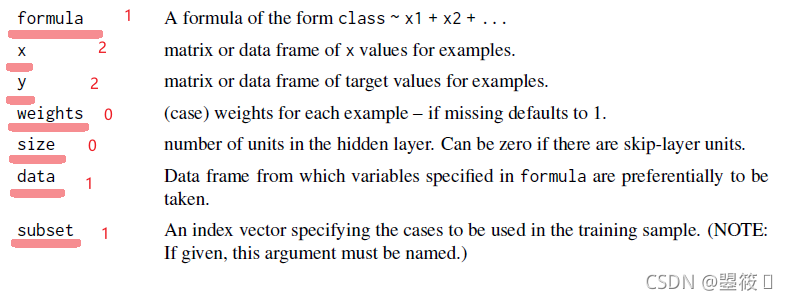
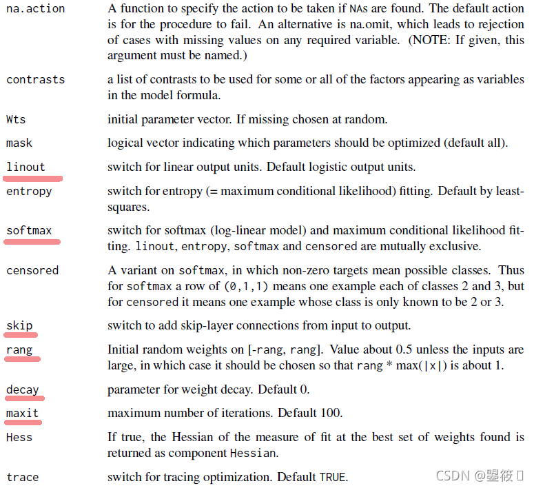
参数说明

先附上文档中的图，等写完后面的原理再回来补
其中划线表示常用，1表示第一种用法需要，2表示第二种用法需要，0表示两种用法都需要

原理学习

Optimization is done via the BFGS method of optim.
从文档中可以得知，该nnet优化方法是BFGS算法，接下来就进行BFGS的学习

未完待续…