梯度下降法与Logistic Regression 及 Matlab 代码

zb12138

已于 2024-04-06 13:51:08 修改

阅读量5.3k

点赞数 9

文章标签： matlab 机器学习开发语言

于 2019-12-21 20:57:36 首次发布

本文链接：https://blog.csdn.net/zb12138/article/details/103639003

版权

梯度下降法与Logistic Regression 及 Matlab 代码

前言

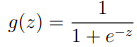
本质是一个求函数最小值问题，这个函数在机器学习中称为Logistic回归，一个通用的求解方法称为梯度下降法。

Logistic回归

Logistic回归用于求解分类问题：
设样本x有n个特征，正负两类y（y = 0 或 1）。现已知m个这样的样本构成样本矩阵X(m * n)及它们对应的类别y(m * 1)（数据）。现需要找到一个判别方法（假设）h，用来预测新样本x0对应的类别y0。

Logistic回归的假设是：

在这里插入图片描述

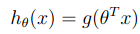
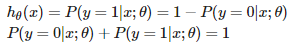
即hθ表示样本为正（y=1）的概率，可以认为
hθ >= 0.5,y=1; hθ < 0.5,y=0;
其中θ是h的参数即我们的求解目标。x表示一个样本，它与θ都是列向量。具体的：

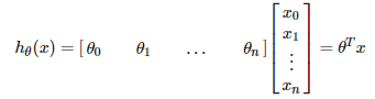
我们强制引入特征x0 = 1，使得θ0成为偏置。

目前有了假设，我们要求解θ ，需要一个标准来评估求解结果，即损失函数。
不用想都知道它应该是训练集分类错误数的增函数。
天才们把它定义为：
在这里插入图片描述
可以验证如果实际y = 1，预测的hθ越大，cost越小，反之（预测错误）cost越大，y = 0也是对的，而且cost >= 0。
至于为什么这样定义，是方便求导以求θ
评估hθ在全体训练集上的总体效果即把m个样本的cost求均值：
在这里插入图片描述
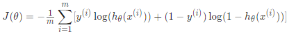
x(i)表示第i个样本，即X(i,:)的转置。

我们的优化目标就是求J(θ)的最小值时θ 为多少。
感谢吴老师的例子，我们在此之上写下这部分matlab代码：

function g = sigmoid(z)
%   SIGMOID Compute sigmoid function
%   g = SIGMOID(z) computes the sigmoid of z.
g = zeros(size(z));
gt = 1./(1 + exp(-z(:)));
g = reshape(gt,size(z));
end

function p = predict(theta, X)
%   PREDICT Predict whether the label is 0 or 1 using learned logistic 
%   regression parameters theta
%   p = PREDICT(theta, X) computes the predictions for X using a 
%   threshold at 0.5 (i.e., if sigmoid(theta'*x) >= 0.5, predict 1)
p = (sigmoid(theta'*X') >= 0.5)';
end

function [J, grad] = costFunction(theta, X, y)
%   COSTFUNCTION Compute cost and gradient for logistic regression
%   J = COSTFUNCTION(theta, X, y) computes the cost of using theta as the
%   parameter for logistic regression and the gradient of the cost
m = length(y); % number of training examples
h = sigmoid(theta'*X');%h is row vector
J = (-log(h)*y - log(1-h)*(1-y)) /m ;
end
grad = ((h - y')*X /m)' ;
end

梯度下降法

我们知道函数梯度的方向是函数增最快的方向，其增长率等于梯度的模。反之，我们每次向梯度的发方向更新θ就可能找到极小（最小）值点，在越接近极值时函数变化越慢，模越小，θ变化就越小，这样才能保证收敛。
此处我们需要求J(θ)的梯度，不信可以自己算，J(θ)的梯度如下：
在这里插入图片描述
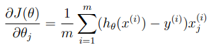
非常的巧妙，这和线性回归的一模一样。
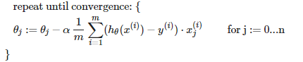
最后梯度下降就是这样，向梯度反方向按α（学习率）比例更新θ直到收敛。

这部分matlab代码如下(J(θ)的梯度计算见costFunction)：

function [theta_A,cost_A] = GradientDescent(theta,learning_rate,X,y)
cost = 1;
cost_A = 1;%cost历史
theta_A = theta;%theta历史
while(cost>=0.2036) %此参数可调，目前就这样写吧，因为还没想好怎么判断收敛orz...
    [cost,grad] = costFunction(theta, X, y);
    theta = theta - learning_rate * grad;
    cost_A = [cost_A cost];
    theta_A = [theta_A theta]; 
 end
end

其实现在就可以开心计算了。

例子1，固定学习率

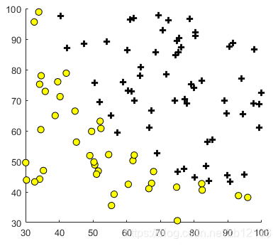
下面的例子有个100个样本,2个特征（m=100，n=2）,要求解的是一个3*1的θ
样本 ex2data1.txt：
34.62365962451697,78.0246928153624,0
30.28671076822607,43.89499752400101,0
35.84740876993872,72.90219802708364,0
60.18259938620976,86.30855209546826,1
79.0327360507101,75.3443764369103,1
45.08327747668339,56.3163717815305,0
61.10666453684766,96.51142588489624,1
75.02474556738889,46.55401354116538,1
76.09878670226257,87.42056971926803,1
84.43281996120035,43.53339331072109,1
95.86155507093572,38.22527805795094,0
75.01365838958247,30.60326323428011,0
82.30705337399482,76.48196330235604,1
69.36458875970939,97.71869196188608,1
39.53833914367223,76.03681085115882,0
53.9710521485623,89.20735013750205,1
69.07014406283025,52.74046973016765,1
67.94685547711617,46.67857410673128,0
70.66150955499435,92.92713789364831,1
76.97878372747498,47.57596364975532,1
67.37202754570876,42.83843832029179,0
89.67677575072079,65.79936592745237,1
50.534788289883,48.85581152764205,0
34.21206097786789,44.20952859866288,0
77.9240914545704,68.9723599933059,1
62.27101367004632,69.95445795447587,1
80.1901807509566,44.82162893218353,1
93.114388797442,38.80067033713209,0
61.83020602312595,50.25610789244621,0
38.78580379679423,64.99568095539578,0
61.379289447425,72.80788731317097,1
85.40451939411645,57.05198397627122,1
52.10797973193984,63.12762376881715,0
52.04540476831827,69.43286012045222,1
40.23689373545111,71.16774802184875,0
54.63510555424817,52.21388588061123,0
33.91550010906887,98.86943574220611,0
64.17698887494485,80.90806058670817,1
74.78925295941542,41.57341522824434,0
34.1836400264419,75.2377203360134,0
83.90239366249155,56.30804621605327,1
51.54772026906181,46.85629026349976,0
94.44336776917852,65.56892160559052,1
82.36875375713919,40.61825515970618,0
51.04775177128865,45.82270145776001,0
62.22267576120188,52.06099194836679,0
77.19303492601364,70.45820000180959,1
97.77159928000232,86.7278223300282,1
62.07306379667647,96.76882412413983,1
91.56497449807442,88.69629254546599,1
79.94481794066932,74.16311935043758,1
99.2725269292572,60.99903099844988,1
90.54671411399852,43.39060180650027,1
34.52451385320009,60.39634245837173,0
50.2864961189907,49.80453881323059,0
49.58667721632031,59.80895099453265,0
97.64563396007767,68.86157272420604,1
32.57720016809309,95.59854761387875,0
74.24869136721598,69.82457122657193,1
71.79646205863379,78.45356224515052,1
75.3956114656803,85.75993667331619,1
35.28611281526193,47.02051394723416,0
56.25381749711624,39.26147251058019,0
30.05882244669796,49.59297386723685,0
44.66826172480893,66.45008614558913,0
66.56089447242954,41.09209807936973,0
40.45755098375164,97.53518548909936,1
49.07256321908844,51.88321182073966,0
80.27957401466998,92.11606081344084,1
66.74671856944039,60.99139402740988,1
32.72283304060323,43.30717306430063,0
64.0393204150601,78.03168802018232,1
72.34649422579923,96.22759296761404,1
60.45788573918959,73.09499809758037,1
58.84095621726802,75.85844831279042,1
99.82785779692128,72.36925193383885,1
47.26426910848174,88.47586499559782,1
50.45815980285988,75.80985952982456,1
60.45555629271532,42.50840943572217,0
82.22666157785568,42.71987853716458,0
88.9138964166533,69.80378889835472,1
94.83450672430196,45.69430680250754,1
67.31925746917527,66.58935317747915,1
57.23870631569862,59.51428198012956,1
80.36675600171273,90.96014789746954,1
68.46852178591112,85.59430710452014,1
42.0754545384731,78.84478600148043,0
75.47770200533905,90.42453899753964,1
78.63542434898018,96.64742716885644,1
52.34800398794107,60.76950525602592,0
94.09433112516793,77.15910509073893,1
90.44855097096364,87.50879176484702,1
55.48216114069585,35.57070347228866,0
74.49269241843041,84.84513684930135,1
89.84580670720979,45.35828361091658,1
83.48916274498238,48.38028579728175,1
42.2617008099817,87.10385094025457,1
99.31500880510394,68.77540947206617,1
55.34001756003703,64.9319380069486,1
74.77589300092767,89.52981289513276,1

数据加载及可视化：

%% Initialization
clear ; close all; clc
%% Load Data
%  The first two columns contains the exam scores and the third column
%  contains the label.
data = load('ex2data1.txt');
X = data(:, [1, 2]); y = data(:, 3);
%% ==================== Part 1: Plotting ====================
%  We start the exercise by first plotting the data to understand the 
%  the problem we are working with.

fprintf(['Plotting data with + indicating (y = 1) examples and o ' ...
         'indicating (y = 0) examples.\n']);
plotData(X, y);
% Put some labels 
hold on;
% Labels and Legend
xlabel('Exam 1 score')
ylabel('Exam 2 score')
% Specified in plot order
legend('Admitted', 'Not admitted')
hold off;

function plotData(X, y)
figure; hold on;
pos = find(y==1); neg = find(y == 0);
% Plot Examples
plot(X(pos, 1), X(pos, 2), 'k+','LineWidth', 2, ...
'MarkerSize', 7);
plot(X(neg, 1), X(neg, 2), 'ko', 'MarkerFaceColor', 'y', ...
'MarkerSize', 7);
hold off;
end

数据可视化结果：
在这里插入图片描述
既然是求最小，当然可以用fminunc：

%% ============= Part 2: Optimizing using fminunc  =============
%  In this exercise, you will use a built-in function (fminunc) to find the
%  optimal parameters theta.
% Initialize fitting parameters
[m, n] = size(X);

% Add intercept term to x and X_test
X = [ones(m, 1) X]; % 强制引入特征x0 = 1，使得θ0成为偏置

% Initialize fitting parameters
initial_theta = zeros(n + 1, 1);

%  Set options for fminunc
options = optimset('GradObj', 'on', 'MaxIter', 400);
%  Run fminunc to obtain the optimal theta
%  This function will return theta and the cost 
[theta, cost] = ...
	fminunc(@(t)(costFunction(t, X, y)), initial_theta, options);
pause;

最优解为
theta = [-25.1613 ; 0.2062 ; 0.2015]
cost = 0.2035
我们用自己写的GradientDescent试试

[theta_A,cost_A] = GradientDescent([0 0 0]',0.001,X,y);%初始点设置为[0;0;0] 学习率0.001大了会翻车！

我们方发现由于固定学习率，此方法非常垃圾，大学习率会导致震荡，小学习率收敛极慢。大概运行2min，实在不确定可以断点看看cost有没有在下降。
这个过程历经600W步，cost变化如下：

plot(cost_A)

在这里插入图片描述
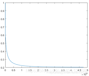
可以看出后面cost收敛非常慢。
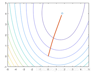
theta（前两个维度）变化如下：

[theataX1,theataX2]= meshgrid( -30:0.01*30:30, -10:0.01*5:1);
J = zeros(size(theataX1));
for i = 1:size(theataX1,1)
        for j = 1:size(theataX1,2)
             theata = [theataX1(i,j),theataX2(i,j),theta(3)]';   
             J(i,j) = costFunction(theata,X,y);
        end
end

contour(theataX1,theataX2,J)
hold on
plot(theta(1),theta(2),'o')
plot(theta_A(1,:),theta_A(2,:),'.-')

在这里插入图片描述
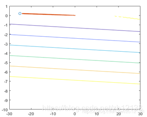
可以看出，等高线非常狭长，这是由于没有正则化引起的。

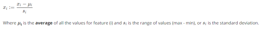
改进1：正则化

数据的不同特征变化范围和对cost影响不一致，导致梯度下降缓慢。我们采取以下方式正则化：
在这里插入图片描述

X_ = [X(:,1) (X(:,2) - mean(X(:,2)))/std(X(:,2)) (X(:,3) - mean(X(:,3)))/std(X(:,3))];

先fminunc更新一下标准答案。
theta = [1.7184;4.0129; 3.7439]
cost = 0.2035
重新试验：

[theta_A,cost_A] = GradientDescent([0 0 0]',0.001,X_,y);

这次仅需要30W步，cost变化形状如上，θ变化如下：
在这里插入图片描述
可以看出，正则化后特征变得均匀。

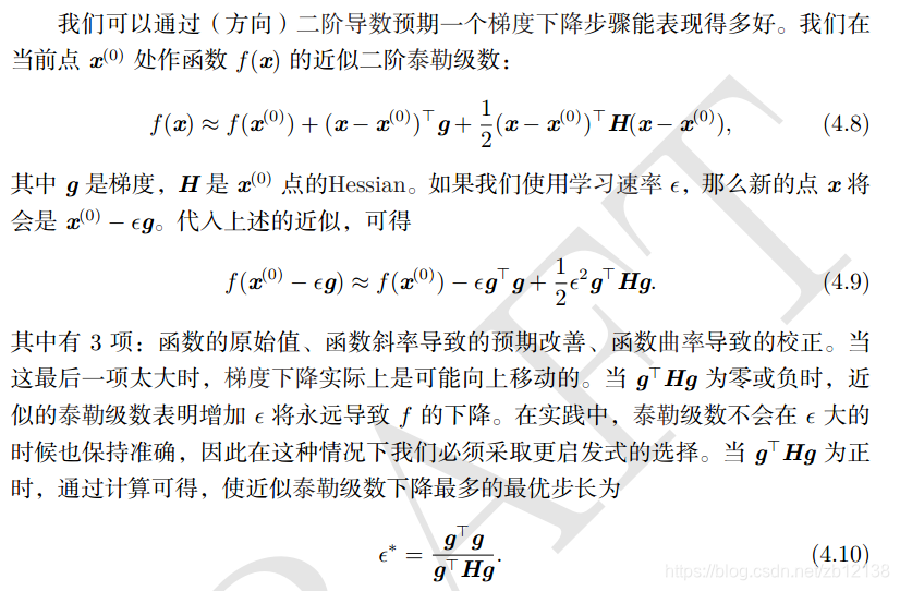
改进2：动态学习率

如果我们每次能动态调整学习率，使得其为最佳，岂不是可以更快。
以下x实则为θ，请勿与样本混淆。
在这里插入图片描述
即g已经在上面costFunction算出来了，grad，只需计算Hessian矩阵H便大功告成了。

在这里插入图片描述
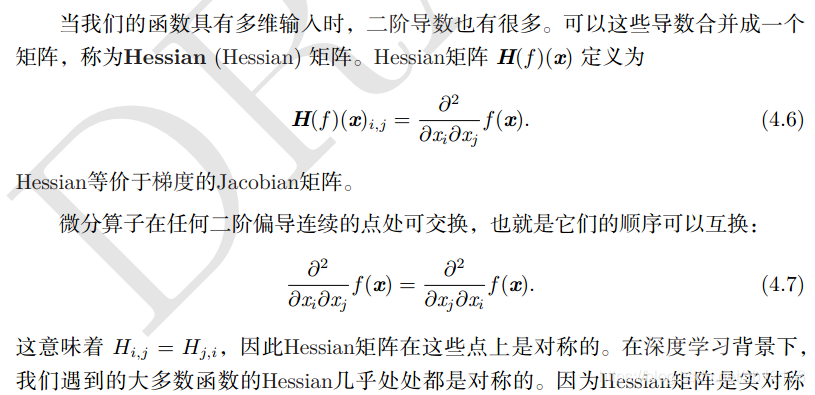
那么在此列Logistic回归中H是个3*3的矩阵，它是多少呢：

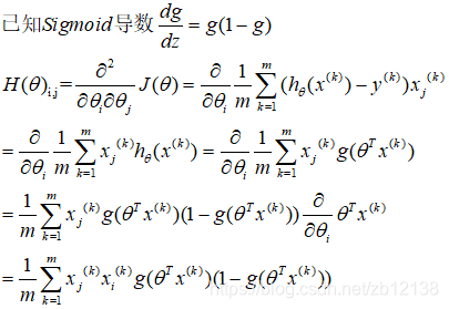
可以看出Hij = Hji 它的确是一个对称矩阵。
下面是matlab实现，有个技巧是每行代表一个样本。

function hessian= Hessian(theta, X)
n = length(theta);
hessian= zeros(n);
h = sigmoid(theta'*X')';
for  j = 1:n
    for i = 1:j
        hessian(i,j) =  mean(X(:,j).* X(:,i).*h.*(1-h));
        hessian(j,i) = hessian(i,j);
    end
end
end

这次我们把收敛条件放严格while(cost>=0.2035)
重写GradientDescent的学习率部分为GradientDescent2：

function [theta_A,cost_A,learning_rate_A] = GradientDescent2(theta,X,y)
cost = 1;
cost_A = 1;
theta_A = theta;
learning_rate_A= 0.001;
while(cost>=0.2035)
    [cost,grad] = costFunction(theta, X, y);
    learning_rate =  grad'*grad/(grad'*Hessian(theta,X)*grad);%动态学习率
    theta = theta - learning_rate * grad;
    learning_rate_A = [learning_rate_A learning_rate]; 
    cost_A = [cost_A cost];
    theta_A = [theta_A theta]; 
 end
 cost
end

测试一下：

[theta_A,cost_A,learning_rate_A] = GradientDescent([0 0 0]',X_,y);

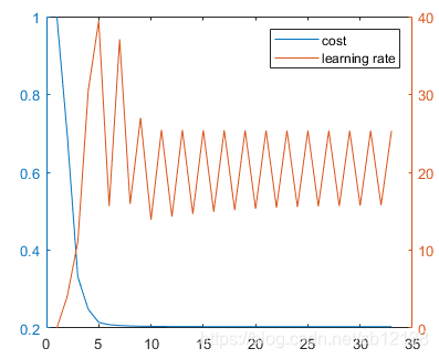
结果只用了33步！
学习率和cost变化如下：
在这里插入图片描述
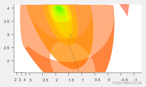
θ变化如下：

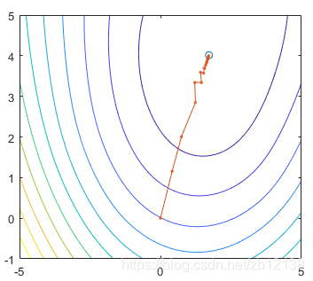
其中的折线似乎不按梯度方向，实际是三维投影在θ前两维的效果。三维空间中θ实际路径如下：

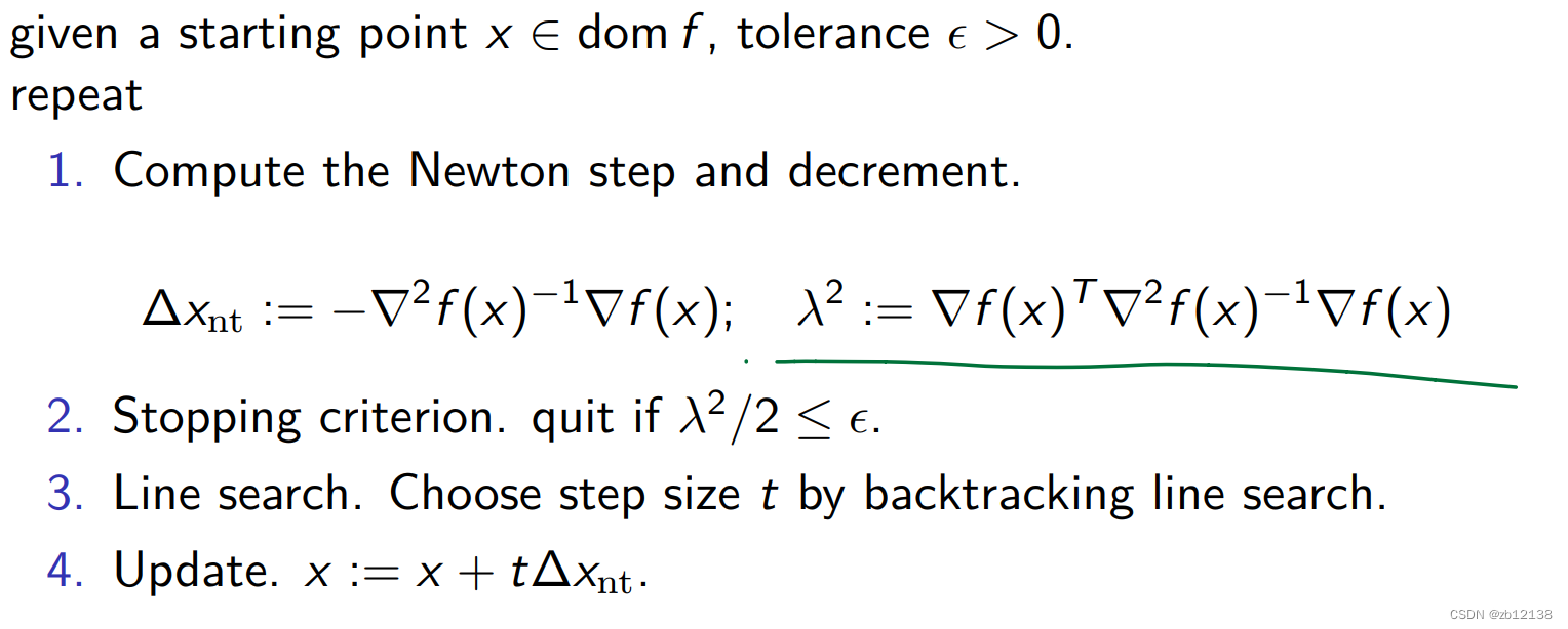
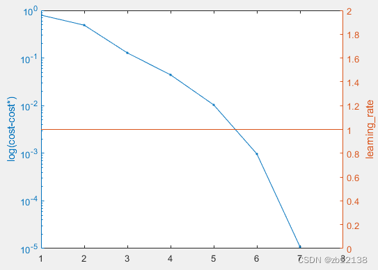
改进3 牛顿法

在这里插入图片描述

function [theta_A,cost_A,learning_rate_A] = NewtonMethod(theta,X,y)
    cost = 1;
    cost_A = 1;
    theta_A = theta;
    learning_rate_A = 1;
    while(cost>=0.2035)
        [cost,grad] = costFunction(theta, X, y);
        delta_theta_nt = -Hessian(theta,X)^(-1)*grad;
        learning_rate= 1;
        [cost_new,g] = costFunction(theta+ learning_rate* delta_theta_nt, X, y);
        while(cost_new>=cost + 1/2*learning_rate*grad'*delta_theta_nt) % backtracking line search
            learning_rate = 1/2*learning_rate;
            [cost_new,g] = costFunction(theta+ learning_rate* delta_theta_nt, X, y);
        end
        theta = theta + learning_rate* delta_theta_nt;
        learning_rate_A = [learning_rate_A learning_rate]; 
        cost_A = [cost_A cost];
        theta_A = [theta_A theta]; 
    end
    disp('final loss')
    disp(cost)
end

平方收敛速度，只用7步！
在这里插入图片描述

在这里插入图片描述

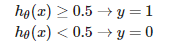
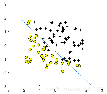
查看分类效果

临界点为h = 0.5 即 θ0+ θ1x1 + θ2x2 =0

plotData(X_(:,2:3),y);
plot_x = [min(X_(:,2))-0.5,  max(X_(:,2))+0.5];
% Calculate the decision boundary line
plot_y = (-1./theta(3)).*(theta(2).*plot_x + theta(1));
hold on
plot(plot_x, plot_y)

在这里插入图片描述

不足

没有收敛判别
在大的初值下会溢出无法运算

完整代码

%% Initialization
clear ; close all; clc
% Load Data
%  The first two columns contains the exam scores and the third column
%  contains the label.

data = load('ex2data1.txt');
X = data(:, [1, 2]); y = data(:, 3);

%% ==================== Part 1: Plotting ====================
%  We start the exercise by first plotting the data to understand the 
%  the problem we are working with.

fprintf(['Plotting data with + indicating (y = 1) examples and o ' ...
         'indicating (y = 0) examples.\n']);

plotData(X, y);

% Put some labels 
hold on;
% Labels and Legend
xlabel('Exam 1 score')
ylabel('Exam 2 score')

% Specified in plot order
legend('Admitted', 'Not admitted')
hold off;

fprintf('\nProgram paused. Press enter to continue.\n');



%% ============ Part 2: Compute Cost and Gradient ============
%  In this part of the exercise, you will implement the cost and gradient
%  for logistic regression. You neeed to complete the code in 
%  costFunction.m

%  Setup the data matrix appropriately, and add ones for the intercept term
[m, n] = size(X);

% Add intercept term to x and X_test
X = [ones(m, 1) X];

% Initialize fitting parameters
initial_theta = zeros(n + 1, 1);

% Compute and display initial cost and gradient
[cost, grad] = costFunction(initial_theta, X, y);

fprintf('Cost at initial theta (zeros): %f\n', cost);
fprintf('Expected cost (approx): 0.693\n');
fprintf('Gradient at initial theta (zeros): \n');
fprintf(' %f \n', grad);
fprintf('Expected gradients (approx):\n -0.1000\n -12.0092\n -11.2628\n');

% Compute and display cost and gradient with non-zero theta
test_theta = [-24; 0.2; 0.2];
[cost, grad] = costFunction(test_theta, X, y);

fprintf('\nCost at test theta: %f\n', cost);
fprintf('Expected cost (approx): 0.218\n');
fprintf('Gradient at test theta: \n');
fprintf(' %f \n', grad);
fprintf('Expected gradients (approx):\n 0.043\n 2.566\n 2.647\n');

fprintf('\nProgram paused. Press enter to continue.\n');

%% ============= Part 3: Optimizing using fminunc  =============
%  In this exercise, you will use a built-in function (fminunc) to find the
%  optimal parameters theta.

%  Set options for fminunc
options = optimset('GradObj', 'on', 'MaxIter', 400);

%  Run fminunc to obtain the optimal theta
%  This function will return theta and the cost 
[theta, cost] = ...
	fminunc(@(t)(costFunction(t, X, y)), initial_theta, options);

% Print theta to screen
fprintf('Cost at theta found by fminunc: %f\n', cost);
fprintf('Expected cost (approx): 0.203\n');
fprintf('theta: \n');
disp('find the optimal solution:')
disp(theta)
fprintf('Expected theta (approx):\n');
fprintf(' -25.161\n 0.206\n 0.201\n');

% Plot Boundary
plotDecisionBoundary(theta, X, y);

% Put some labels 
hold on;
% Labels and Legend
xlabel('Exam 1 score')
ylabel('Exam 2 score')

% Specified in plot order
legend('Admitted', 'Not admitted')
hold off;

fprintf('\nProgram paused. Press enter to continue.\n');

%% ============== Part 4: Predict and Accuracies ==============
%  After learning the parameters, you'll like to use it to predict the outcomes
%  on unseen data. In this part, you will use the logistic regression model
%  to predict the probability that a student with score 45 on exam 1 and 
%  score 85 on exam 2 will be admitted.
%
%  Furthermore, you will compute the training and test set accuracies of 
%  our model.
%
%  Your task is to complete the code in predict.m

%  Predict probability for a student with score 45 on exam 1 
%  and score 85 on exam 2 

prob = sigmoid([1 45 85] * theta);
fprintf(['For a student with scores 45 and 85, we predict an admission ' ...
         'probability of %f\n'], prob);
fprintf('Expected value: 0.775 +/- 0.002\n\n');

% Compute accuracy on our training set
p = (sigmoid(theta'*X') >= 0.5)';

fprintf('Train Accuracy: %f\n', mean(double(p == y)) * 100);
fprintf('Expected accuracy (approx): 89.0\n');
fprintf('\n');

%% ============== Part 5: Original Gradient Descent Method ============== 
% it takes about 2 minutes
% [theta_H,cost_H] = GradientDescent([0 0 0]',0.001,X,y); %The initial point is set to[0;0;0] learning rate 0.001, error if it is too large！
% figure();
% plot(cost_H)
% xlabel('steps'), ylabel('cost')
% viewGradient(theta_H(:,end),theta_H,X,y,-30:0.1*30:30,-10:0.1*5:1);
% disp('find the optimal solution:')
% disp(theta_H(:,end))


%% ============== Part 6: Improvement 1, normalization ============== 
X2 = [X(:,1) (X(:,2) - mean(X(:,2)))/std(X(:,2)) (X(:,3) - mean(X(:,3)))/std(X(:,3))];
[theta_H,cost_H] = GradientDescent([0 0 0]',0.001,X2,y);
figure();
plot(cost_H)
xlabel('steps'), ylabel('cost')
viewGradient(theta_H(:,end),theta_H,X2,y,-5:0.1:5,-1:0.1:5);
disp('find the optimal solution:')
disp(theta_H(:,end))

%% ============== Part 7: Improvement 2, Best Learning Rate by Hessian ============== 
[theta_H,cost_H,learning_rate_H] = GradientDescent2([0 0 0]',X2,y);
figure();
yyaxis left
plot(cost_H,'.-')
ylabel('cost')
yyaxis right
plot(learning_rate_H)
ylabel('learning\_rate')
viewGradient(cost_H,theta_H(:,end),theta_H,X2,y,-5:0.1:5,-1:0.1:5);
viewGradientXZ(cost_H,theta_H(:,end),theta_H,X2,y,-5:0.1:5,0:0.05:5);
viewGradient3D(cost_H,theta_H(:,end),theta_H,X2,y,-5:0.1:5,-1:0.1:5,0:0.05:5);
disp('find the optimal solution:')
disp(theta_H(:,end))

%% ============== Part 8: Newton's method ============== 
[theta_H,cost_H,learning_rate_H] = NewtonMethod([0 0 0]',X2,y);
figure();
yyaxis left
semilogy(cost_H-0.2035,'.-')
ylabel('log(cost-cost*)')
yyaxis right
plot(learning_rate_H)
ylabel('learning\_rate')
viewGradient(cost_H,theta_H(:,end),theta_H,X2,y,-5:0.1:5,-1:0.1:5);
viewGradientXZ(cost_H,theta_H(:,end),theta_H,X2,y,-5:0.1:5,0:0.05:5);
viewGradient3D(cost_H,theta_H(:,end),theta_H,X2,y,-5:0.1:5,-1:0.1:5,0:0.05:5);
disp('find the optimal solution:')
disp(theta_H(:,end))

%%

[cost,grad] = costFunction(theta_H(:,5), X, y);

%%

%% core functions

function g = sigmoid(z)
%SIGMOID Compute sigmoid function
%   g = SIGMOID(z) computes the sigmoid of z.
% You need to return the following variables correctly 
g = zeros(size(z));
% ====================== YOUR CODE HERE ======================
% Instructions: Compute the sigmoid of each value of z (z can be a matrix,
%               vector or scalar).
gt = 1./(1 + exp(-z(:)));
g = reshape(gt,size(z));
% =============================================================

end

function [J, grad] = costFunction(theta, X, y)
%   COSTFUNCTION Compute cost and gradient for logistic regression
%   J = COSTFUNCTION(theta, X, y) computes the cost of using theta as the
%   parameter for logistic regression and the gradient of the cost
m = length(y); % number of training examples
h = sigmoid(theta'*X');%h is row vector
J = (-log(h)*y - log(1-h)*(1-y)) /m ;
grad = ((h - y')*X /m)' ;
end


function [theta_A,cost_A] = GradientDescent(theta,learning_rate,X,y)
    cost = 1;
    cost_A = 1;%cost history
    theta_A = theta;%theta history
    while(cost>=0.2036) % convergence judge
        [cost,grad] = costFunction(theta, X, y);
        theta = theta - learning_rate * grad;
        cost_A = [cost_A cost];
        theta_A = [theta_A theta]; 
     end
end


function [theta_A,cost_A,learning_rate_A] = GradientDescent2(theta,X,y)
    cost = 1;
    cost_A = 1;
    theta_A = theta;
    learning_rate_A= 0.001;
    while(cost>=0.2035)
        [cost,grad] = costFunction(theta, X, y);
        learning_rate =  grad'*grad/(grad'*Hessian(theta,X)*grad);% dynamic learning rate
        theta = theta - learning_rate * grad;
        learning_rate_A = [learning_rate_A learning_rate]; 
        cost_A = [cost_A cost];
        theta_A = [theta_A theta]; 
    end
    disp('final loss')
    disp(cost)
end

function [theta_A,cost_A,learning_rate_A] = NewtonMethod(theta,X,y)
    cost = 1;
    cost_A = 1;
    theta_A = theta;
    learning_rate_A = 1;
    lamda2 = 1;
    while(lamda2/2>=10^(-10))
        [cost,grad] = costFunction(theta, X, y);
        delta_theta_nt = -Hessian(theta,X)^(-1)*grad;
        learning_rate= 1;
        [cost_new,g] = costFunction(theta+ learning_rate* delta_theta_nt, X, y);
        while(learning_rate>0 && cost_new>=cost + 1/2*learning_rate*grad'*delta_theta_nt) % backtracking line search
            learning_rate = 1/2*learning_rate;
            [cost_new,g] = costFunction(theta+ learning_rate* delta_theta_nt, X, y);
        end
        theta = theta + learning_rate* delta_theta_nt;
        lamda2 = -g'*delta_theta_nt;
        learning_rate_A = [learning_rate_A learning_rate]; 
        cost_A = [cost_A cost];
        theta_A = [theta_A theta]; 
    end
    disp('final loss')
    disp(cost)
end

function hessian= Hessian(theta, X)
n = length(theta);
hessian= zeros(n);
h = sigmoid(theta'*X')';
for  j = 1:n
    for i = 1:j
        hessian(i,j) =  mean(X(:,j).* X(:,i).*h.*(1-h));
        hessian(j,i) = hessian(i,j);
    end
end
end


%% helper functions

function plotData(X, y)
figure; hold on;
pos = find(y==1); neg = find(y == 0);
% Plot Examples
plot(X(pos, 1), X(pos, 2), 'k+','LineWidth', 2, ...
'MarkerSize', 7);
plot(X(neg, 1), X(neg, 2), 'ko', 'MarkerFaceColor', 'y', ...
'MarkerSize', 7);
hold off;
end

function viewGradient(cost_H,theta_target,theta_history,X,y, viewX,viewY)
    [thetaX1,thetaX2]= meshgrid(viewX,viewY);
    J = zeros(size(thetaX1));
    for i = 1:size(thetaX1,1)
            for j = 1:size(thetaX1,2)
                 theta = [thetaX1(i,j),thetaX2(i,j),theta_target(3)]';   
                 J(i,j) = costFunction(theta,X,y);
            end
    end
    figure();
    contour(thetaX1,thetaX2,J,cost_H)
    hold on
    plot(theta_target(1),theta_target(2),'o')
    plot(theta_history(1,:),theta_history(2,:),'.-')
    xlabel('theta1')
    ylabel('theta2')
    hold off
end

function viewGradientXZ(cost_H,theta_target,theta_history,X,y, viewX,viewZ)
    [thetaX1,thetaX2]= meshgrid(viewX,viewZ);
    J = zeros(size(thetaX1));
    for i = 1:size(thetaX1,1)
            for j = 1:size(thetaX1,2)
                 theta = [thetaX1(i,j),theta_target(2),thetaX2(i,j)]';   
                 J(i,j) = costFunction(theta,X,y);
            end
    end
    figure();
    contour(thetaX1,thetaX2,J,sort(cost_H))
    hold on
    plot(theta_target(1),theta_target(3),'o')
    plot(theta_history(1,:),theta_history(3,:),'.-')
    xlabel('theta1')
    ylabel('theta3')
    hold off
end

function viewGradient3D(cost_H,theta_target,theta_history,X,y, viewX,viewY,viewZ)
    [thetaX1,thetaX2,thetaX3]= meshgrid(viewX,viewY,viewZ);
        J = zeros(size(thetaX1));
        for i = 1:size(thetaX1,1)
                for j = 1:size(thetaX1,2)
                    for k = 1:size(thetaX1,3)
                         theta = [thetaX1(i,j,k),thetaX2(i,j,k),thetaX3(i,j,k)]';   
                         J(i,j,k) = costFunction(theta,X,y);
                    end
                end
        end
    figure();
    hold on
    V = cost_H;
    c = hsv(length(V));
    for i = 1:length(V)
        v = V(i);
    s = isosurface(thetaX1,thetaX2,thetaX3,J,v,ones(size(J))*v);
    p = patch(s);
    isonormals(thetaX1,thetaX2,thetaX3,J,p)
    view(3);
    set(p,'FaceColor',c(i,:));  
    set(p,'EdgeColor','none');
    set(p,'FaceAlpha',0.5);
    % camlight;
    % lighting gouraud;
    end
    axis equal
    plot3(theta_history(1,:),theta_history(2,:),theta_history(3,:),'.-')
    plot3(theta_target(1),theta_target(2),theta_target(3),'o')
    hold off
end

function plotDecisionBoundary(theta, X, y)
%PLOTDECISIONBOUNDARY Plots the data points X and y into a new figure with
%the decision boundary defined by theta
%   PLOTDECISIONBOUNDARY(theta, X,y) plots the data points with + for the 
%   positive examples and o for the negative examples. X is assumed to be 
%   a either 
%   1) Mx3 matrix, where the first column is an all-ones column for the 
%      intercept.
%   2) MxN, N>3 matrix, where the first column is all-ones

% Plot Data
plotData(X(:,2:3), y);
hold on

if size(X, 2) <= 3
    % Only need 2 points to define a line, so choose two endpoints
    plot_x = [min(X(:,2))-2,  max(X(:,2))+2];

    % Calculate the decision boundary line
    plot_y = (-1./theta(3)).*(theta(2).*plot_x + theta(1));

    % Plot, and adjust axes for better viewing
    plot(plot_x, plot_y)
    
    % Legend, specific for the exercise
    legend('Admitted', 'Not admitted', 'Decision Boundary')
    axis([30, 100, 30, 100])
else
    % Here is the grid range
    u = linspace(-1, 1.5, 50);
    v = linspace(-1, 1.5, 50);

    z = zeros(length(u), length(v));
    % Evaluate z = theta*x over the grid
    for i = 1:length(u)
        for j = 1:length(v)
            z(i,j) = mapFeature(u(i), v(j))*theta;
        end
    end
    z = z'; % important to transpose z before calling contour

    % Plot z = 0
    % Notice you need to specify the range [0, 0]
    contour(u, v, z, [0, 0], 'LineWidth', 2)
end
hold off

end