机器学习课程代码【线性回归与梯度下降】

1.warmUpExercise()

function A = warmUpExercise()
%UNTITLED5 Summary of this function goes here
%   Detailed explanation goes here
A = eye(5);

2.Plotting

data = load('ex1data1.txt'); % read comma separated data
x = data(:, 1); y = data(:, 2);
m = length(y); % number of training examples

plot(x, y, 'rx', 'MarkerSize', 10); % Plot the data
ylabel('Profit in $10,000s'); % Set the y−axis label
xlabel('Population of City in 10,000s'); % Set the x−axis label

3.代价函数的计算

先看公式：  

data = load('ex1data1.txt'); % read comma separated data  先把数据加载进来
x = data(:, 1); y = data(:, 2);%分别取第一列第二列
m = length(y); 
X = [ones(m, 1), data(:,1)];% Add a column of ones to x  X是两列一行的矩阵，第一列全是1,第二列是所有的x即data数据的第一列
theta = zeros(2, 1); % initialize fitting parameters 先给θ0和θ1赋值，两行一列的0矩阵，对应两个θ参数
%iterations = 1500;迭代次数
alpha = 0.01;
fprintf('\nTesting the cost function ...\n')
% compute and display initial cost
J = 0;
J=sum((X*theta-y).^2)/(2*m); %看公式
fprintf('With theta = [0 ; 0]\nCost computed = %f\n', J); %计算结果
fprintf('Expected cost value (approx) 32.07\n');
theta=[-1 ; 2];    %换参数试试
J=sum((X*theta-y).^2)/(2*m);
fprintf('\nWith theta = [-1 ; 2]\nCost computed = %f\n', J);
fprintf('Expected cost value (approx) 54.24\n');

结果：

4.梯度下降

https://blog.csdn.net/zbl1243/article/details/80790075   文章最后有上式推导

代码接着代价函数继续：

data = load('ex1data1.txt'); % read comma separated data  先把数据加载进来
x = data(:, 1); y = data(:, 2);%分别取第一列第二列
m = length(y); 

X = [ones(m, 1), data(:,1)];% Add a column of ones to x  X是两列一行的矩阵，第一列全是1,第二列是所有的x即data数据的第一列

theta = zeros(2, 1); % initialize fitting parameters 先给θ0和θ1赋值，两行一列的0矩阵，对应两个θ参数
%iterations = 1500;迭代次数
alpha = 0.01;
fprintf('\nTesting the cost function ...\n')
% compute and display initial cost
J = 0;
J=sum((X*theta-y).^2)/(2*m); %看公式

fprintf('With theta = [0 ; 0]\nCost computed = %f\n', J); %计算结果
fprintf('Expected cost value (approx) 32.07\n');


theta=[-1 ; 2];    %换参数试试
%J = computeCost(X, y, [-1 ; 2]);
J=sum((X*theta-y).^2)/(2*m);
fprintf('\nWith theta = [-1 ; 2]\nCost computed = %f\n', J);
fprintf('Expected cost value (approx) 54.24\n');

% -------------------------------------------------------------梯度下降--------------------------------------------------


for iter = 1:iterations  %迭代


    x=X(:,2);   %所有的x
    theta0=theta(1);
    theta1=theta(2);
    
    theta0=theta0-alpha/m*sum(X*theta-y);
    theta1=theta1-alpha/m*sum((X*theta-y).*x);
    
    theta=[theta0;theta1];
   
    J=sum((X*theta-y).^2)/(2*m);
    

end

fprintf('J:%f\n',J);%看看最后的J是不是靠近0

% print theta to screen
fprintf('Theta found by gradient descent:\n');
fprintf('%f\n', theta);
fprintf('Expected theta values (approx)\n');
fprintf(' -3.6303\n  1.1664\n\n');

% Plot the linear fit
hold on; % keep previous plot visible 多图共存
plot(X(:,2), y, 'rx', 'MarkerSize', 10); % Plot the data
plot(X(:,2), X*theta, '-')

legend('Training data', 'Linear regression')
hold off % don't overlay any more plots on this figure

5.画图

接上面

theta0_vals = linspace(-10, 10, 100)
theta1_vals = linspace(-1, 4, 100);

% initialize J_vals to a matrix of 0's
J_vals = zeros(length(theta0_vals), length(theta1_vals));

% Fill out J_vals
for i = 1:length(theta0_vals)
    for j = 1:length(theta1_vals)
	  t = [theta0_vals(i); theta1_vals(j)];
      J=sum((X*t-y).^2)/(2*m);
	  J_vals(i,j) = J;
    end
end


% Because of the way meshgrids work in the surf command, we need to
% transpose J_vals before calling surf, or else the axes will be flipped
J_vals = J_vals';   %还是不懂为什么要转置 emmmmmm theta1_vals theta0_vals都是1行100列，J_vals是100x100

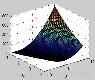
% Surface plot
figure;

surf(theta0_vals, theta1_vals, J_vals)
xlabel('\theta_0'); ylabel('\theta_1');

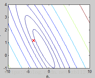
% Contour plot
figure;
% Plot J_vals as 15 contours spaced logarithmically between 0.01 and 100
contour(theta0_vals, theta1_vals, J_vals, logspace(-2, 3, 20))
xlabel('\theta_0'); ylabel('\theta_1');
hold on;
plot(theta(1), theta(2), 'rx', 'MarkerSize', 10, 'LineWidth', 2);