机器学习的初学者入门：神经网络之简介

一篇文章简单介绍神经网络如何工作的，以及如何从零开始在 Python 中实现一个神经网络。
A simple explanation of how they work and how to implement one from scratch in Python.

原文地址：https://victorzhou.com/blog/intro-to-neural-networks/。

听起来可能有点让你惊讶，那就是**神经网络并不复杂！**虽然“神经网络”本身是一个热词（buzzword），但实际上比人们想象中来得简单。
Here’s something that might surprise you: neural networks aren’t that complicated! The term “neural network” gets used as a buzzword a lot, but in reality they’re often much simpler than people imagine.

本文正是针对那些机器学习零基础的初学者，在了解神经网络工作原理的同时，实现一个 Python 的神经网络。
This post is intended for complete beginners and assumes ZERO prior knowledge of machine learning. We’ll understand how neural networks work while implementing one from scratch in Python.

咱开始吧！Let’s get started!

构建区块：神经元 Building Blocks: Neurons

首先说说神经网络的基础单元：神经元（neuron）。一个神经元有输入，进行相关数学运算，然后返回结果。如下这个神经元有两个输入：
First, we have to talk about neurons, the basic unit of a neural network. A neuron takes inputs, does some math with them, and produces one output. Here’s what a 2-input neuron looks like:

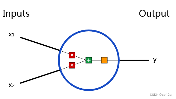
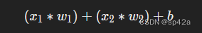
这里发生了三件事情。第一，每个输入乘于一个权重（weight，上图的红色部分）：

第二，所有已配权重的输入进行相加，然后加上一个偏差（bias） b（上图的黄色部分）：

最后，将求和的结果输入一个激活函数（activation function，上图的橙色部分）。

激活函数在神经网络中被用来处理无界的输入数据，并将其转换为具有良好可预测形式的输出。一个常用的激活函数是 sigmoid 函数。（译注：无界 表示输入的数值范围不受限制，可以是任意实数；良好可预测形式 表示输出的数值应该是有界的，并且服从一定的规律，便于后续计算。）
The activation function is used to turn an unbounded input into an output that has a nice, predictable form. A commonly used activation function is the sigmoid function:

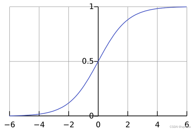
sigmoid 函数的输出值仅在 (0, 1) 之间。我们可以把它想象成一个压缩函数，将所有实数范围 (负无穷到正无穷) 压缩到 (0, 1) 之间。对于非常大的负数，sigmoid 函数会将其输出接近于 0；对于非常大的正数，sigmoid 函数会将其输出接近于 1。
The sigmoid function only outputs numbers in the range (0,1). You can think of it as compressing (−∞,+∞) to (0,1) - big negative numbers become ~0, and big positive numbers become ~1.

举个简单的例子 A Simple Example

假設我們有一個 2-輸入的神經元，它使用 sigmoid 激活函数并具有以下参数：w=[0,1] b=4
Assume we have a 2-input neuron that uses the sigmoid activation function and has the following parameters: w=[0,1] b=4。

w=[0,1] 只是 w1=0,w2=1 的向量形式。现在，我们给神经元输入一个 x=[2,3]。我们将使用点积来更简洁地表示：
w=[0,1] is just a way of writing w1=0,w2=1 in vector form. Now, let’s give the neuron an input of x=[2,3]. We’ll use the dot product to write things more concisely:

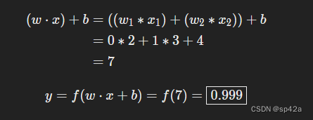
(w⋅x)+b=((w1∗x1)+(w2∗x2))+b=0∗2+1∗3+4=7
 y=f(w⋅x+b)=f(7)=0.999

神经元输出 0.999 给定输入x=[2,3]。 这就是了！ 将输入向前传递以获得输出的过程称为前馈 （feedforward）。

The neuron outputs 0.999 given the inputs x=[2,3]. That’s it! This process of passing inputs forward to get an output is known as feedforward.

写一个神经元 Coding a Neuron

是时候实现神经元了。我们用 NumPy 来搞定，一个强大而且流行的 Python 库，以帮助我们进行计算：
Time to implement a neuron! We’ll use NumPy, a popular and powerful computing library for Python, to help us do math:

import numpy as np

def sigmoid(x):
  # Our activation function: f(x) = 1 / (1 + e^(-x))
  return 1 / (1 + np.exp(-x))

class Neuron:
  def __init__(self, weights, bias):
    self.weights = weights
    self.bias = bias

  def feedforward(self, inputs):
    # 权重输入，添加偏差，然后使用激活函数 Weight inputs, add bias, then use the activation function
    total = np.dot(self.weights, inputs) + self.bias
    return sigmoid(total)

weights = np.array([0, 1]) # w1 = 0, w2 = 1
bias = 4                   # b = 4
n = Neuron(weights, bias)

x = np.array([2, 3])       # x1 = 2, x2 = 3
print(n.feedforward(x))    # 0.9990889488055994

结果如同例子所示！
Recognize those numbers? That’s the example we just did! We get the same answer of 0.9990.999.

组合多个神经元到一个神经网络 Combining Neurons into a Neural Network

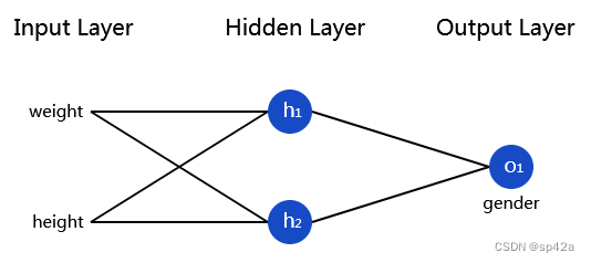
一个神经网络就是多个神经元连接起来的集合。一个简单的神经网络看起来像这样的：
A neural network is nothing more than a bunch of neurons connected together. Here’s what a simple neural network might look like:

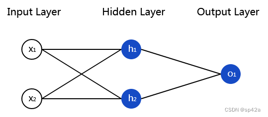
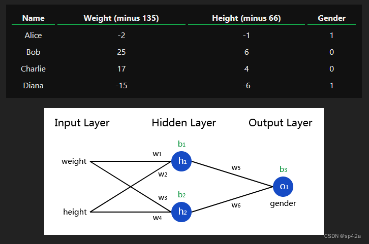
这个网络有两个输入，一个有两个神经元的隐藏层（h1、h2），以及一个带有一个神经元的输出 o1。注意 o1 的输入是 h1 及 h2 的输出，这样就构成了一个网络。
This network has 2 inputs, a hidden layer with 2 neurons (h1​ and h2​), and an output layer with 1 neuron (o1​). Notice that the inputs for o1​ are the outputs from h1​ and h2​ - that’s what makes this a network.

隐藏层指的是介乎于第一个输入层与最后一个输出层之间任意层。这里允许有多个隐藏的层！
A hidden layer is any layer between the input (first) layer and output (last) layer. There can be multiple hidden layers!

前馈的一个例子 An Example: Feedforward

还是使用上面那张网络图，假设所有的神经元有同样的输入权重w=[0,1]，同样的偏差b=0，同样的 sigmoid 激活函数。h1，h2，o1 分别代表它们所表示的神经元的输出。
Let’s use the network pictured above and assume all neurons have the same weights w=[0,1], the same bias b=0, and the same sigmoid activation function. Let h1,h2,o1​ denote the outputs of the neurons they represent.

如果输入x=[2,3] 会发生什么？
What happens if we pass in the input x=[2,3]?

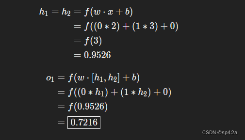
h1=h2=f(w⋅x+b)=f((0∗2)+(1∗3)+0)=f(3)=0.9526
o1=f(w⋅[h1,h2]+b)=f((0∗h1)+(1∗h2)+0)=f(0.9526)=0.7216

输入x=[2,3]神经网络会输出0.7216，非常简单的是吧?
The output of the neural network for input x=[2,3] is 0.7216. Pretty simple, right?

神经网络可以拥有任意数量的层，每层中的神经元数量也可以任意。基本思想保持不变：将输入向前馈送通过网络中的神经元，以获得最终的输出。为了简单起见，我们将继续使用上面图片中的网络来完成本文的其余部分。
A neural network can have any number of layers with any number of neurons in those layers. The basic idea stays the same: feed the input(s) forward through the neurons in the network to get the output(s) at the end. For simplicity, we’ll keep using the network pictured above for the rest of this post.

编码一个神经网络的前馈 Coding a Neural Network: Feedforward

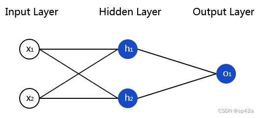
现在为我们的神经网络来实现前馈。这是一张神经网络的参考图：
Let’s implement feedforward for our neural network. Here’s the image of the network again for reference:

import numpy as np

# ... code from previous section here

class OurNeuralNetwork:
  '''
  A neural network with:
    - 2 inputs
    - a hidden layer with 2 neurons (h1, h2)
    - an output layer with 1 neuron (o1)
  Each neuron has the same weights and bias:
    - w = [0, 1]
    - b = 0
  '''
  def __init__(self):
    weights = np.array([0, 1])
    bias = 0

    # 这里的神经元类来自前面的部分。The Neuron class here is from the previous section
    self.h1 = Neuron(weights, bias)
    self.h2 = Neuron(weights, bias)
    self.o1 = Neuron(weights, bias)

  def feedforward(self, x):
    out_h1 = self.h1.feedforward(x)
    out_h2 = self.h2.feedforward(x)

    # o1的输入是来自h1和h2的输出。The inputs for o1 are the outputs from h1 and h2
    out_o1 = self.o1.feedforward(np.array([out_h1, out_h2]))

    return out_o1

network = OurNeuralNetwork()
x = np.array([2, 3])
print(network.feedforward(x)) # 0.7216325609518421

We got 0.72160.7216 again! Looks like it works.

训练一个神经网络，第一部分 Training a Neural Network, Part 1

假如我们有这些测量数据：
Say we have the following measurements:

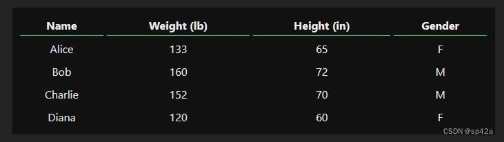
让我们训练我们的网络，根据一个人的体重和身高来预测他们的性别：
Let’s train our network to predict someone’s gender given their weight and height:

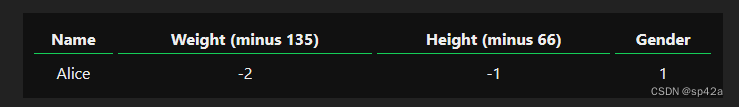
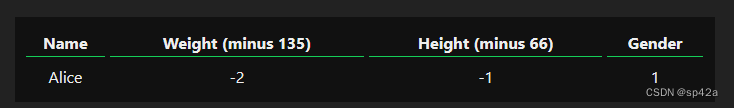
我们将用0表示男性，用1表示女性，我们还将调整数据以使其更易于使用：

We’ll represent Male with a 0 and Female with a 1, and we’ll also shift the data to make it easier to use:

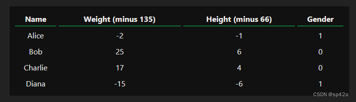
我任意选择了偏移量（135 和 66）使数字看起来更整齐。通常情况下，你会通过均值来进行偏移。
I arbitrarily chose the shift amounts (135 and 66) to make the numbers look nice. Normally, you’d shift by the mean.

损失 Loss

在训练我们的网络之前，我们首先需要一种方法来量化它的表现如何，以便它可以尝试做得更好。这就是损失的作用。
Before we train our network, we first need a way to quantify how “good” it’s doing so that it can try to do “better”. That’s what the loss is.

我们将使用均方误差（MSE）损失：
We’ll use the mean squared error (MSE) loss:

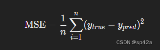
MSE=1n∑i=1n(ytrue−ypred)2

让我们逐步分解一下：Let’s break this down:

• n 是样本的数量，这里是 44（Alice，Bob，Charlie，Diana）。n is the number of samples, which is 4 (Alice, Bob, Charlie, Diana).
• y 代表被预测的变量，即性别。y represents the variable being predicted, which is Gender.
• ytrue 是变量的真实值（“正确答案”）。例如，Alice 的 ytrue 是1（女性）。ytrue is the true value of the variable (the “correct answer”). For example, ytrueytrue​ for Alice would be 1 (Female).
• ypred 是变量的预测值。它是我们的网络输出的值。ypred​ is the predicted value of the variable. It’s whatever our network outputs.

(ytrue−ypred)2 被称为平方误差。我们的损失函数只是对所有平方误差取平均值（因此称为均方误差）。我们的预测越准确，损失就越低！
(ytrue−ypred)2 is known as the squared error. Our loss function is simply taking the average over all squared errors (hence the name mean squared error). The better our predictions are, the lower our loss will be!

更好的预测 = 更低的损失。Better predictions = Lower loss.

训练一个网络 = 尝试最小化其损失。Training a network = trying to minimize its loss.

计算损失的一个例子 An Example Loss Calculation

假设我们的网络总是输出0 - 换句话说，它确信所有人都是男性。我们的损失会是多少呢？
Let’s say our network always outputs 0 - in other words, it’s confident all humans are Male. What would our loss be?

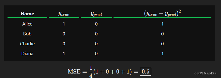
MSE=14(1+0+0+1)=0.5

MSE 损失代码 Code: MSE Loss

下面是我们用于计算损失的代码：
Here’s some code to calculate loss for us:

import numpy as np

def mse_loss(y_true, y_pred):
  # y_true 和 y_pred 是长度相同的 NumPy 数组。y_true and y_pred are numpy arrays of the same length.
  return ((y_true - y_pred) ** 2).mean()

y_true = np.array([1, 0, 0, 1])
y_pred = np.array([0, 0, 0, 0])

print(mse_loss(y_true, y_pred)) # 0.5

如果你不明白这段代码为什么有效，可以阅读一下NumPy快速入门中的数组操作部分。
If you don’t understand why this code works, read the NumPy quickstart on array operations.

好的，继续前进吧！Nice. Onwards!

训练一个神经网络，第二部分 Training a Neural Network, Part 2

我们现在有一个明确的目标：最小化神经网络的损失。我们知道可以通过改变网络的权重和偏置来影响其预测结果，但我们如何以降低损失的方式进行调整呢？
We now have a clear goal: minimize the loss of the neural network. We know we can change the network’s weights and biases to influence its predictions, but how do we do so in a way that decreases loss?

这一部分涉及到一些多元微积分。如果你对微积分不太熟悉，可以跳过数学部分。
This section uses a bit of multivariable calculus. If you’re not comfortable with calculus, feel free to skip over the math parts.

为简单起见，让我们假装数据集中只有 Alice。
For simplicity, let’s pretend we only have Alice in our dataset:

那么均方误差损失就只是 Alice 的平方误差：
Then the mean squared error loss is just Alice’s squared error:

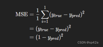
MSE=11∑i=11(ytrue−ypred)2=(ytrue−ypred)2=(1−ypred)2

将损失看作是权重和偏差的函数的另一种方式。让我们给网络中的每个权重和偏差进行标记：
Another way to think about loss is as a function of weights and biases. Let’s label each weight and bias in our network:

那么，我们可以将损失写成一个多变量函数：
Then, we can write loss as a multivariable function:

L(w1,w2,w3,w4,w5,w6,b1,b2,b3)

想象一下，如果我们想要微调 w1，如果我们改变了 w1，损失 LL 会如何变化？这是偏导数 ∂L/∂w1 可以回答的问题。那么我们如何计算它呢？
Imagine we wanted to tweak w1. How would loss L change if we changed w1​? That’s a question the partial derivative ∂L/∂w1​ can answer. How do we calculate it?

这里的数学开始变得更加复杂。**不要气馁！**我建议拿起笔和纸跟着走 - 这会帮助你理解。
Here’s where the math starts to get more complex. Don’t be discouraged! I recommend getting a pen and paper to follow along - it’ll help you understand.

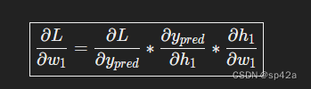
首先，让我们用 ∂ypred/∂w1 来重新表达偏导数：
To start, let’s rewrite the partial derivative in terms of ∂ypred/∂w1​​ instead:

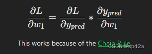
这是因为链式法则。This works because of the Chain Rule.

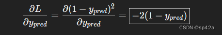
我们可以计算 ∂L/∂ypred 因为我们之前计算了 L=(1−ypred)2：
We can calculate ∂L/∂ypred because we computed L=(1−ypred)2 above:

现在，让我们弄清楚如何处理 ∂ypred/∂w1 就像之前一样，设 h1，h2，o1 为它们所代表的神经元的输出。然后
Now, let’s figure out what to do with ∂ypred/∂w1 Just like before, let h1,h2,o1 be the outputs of the neurons they represent. Then

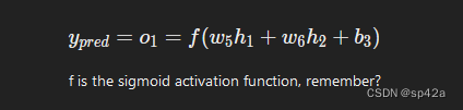
f 是 Sigmoid 激活函数，记得吗？
f is the sigmoid activation function, remember?

由于 w1 只影响 h1（不影响 h2），我们可以写成：
Since w1​ only affects h1​ (not h2​), we can write

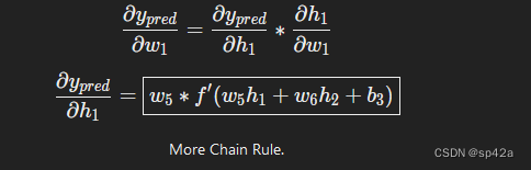
更多的链式法则 More Chain Rule.

我们对 ∂h1/∂w1 做同样的事情：We do the same thing for∂h1/∂w1:

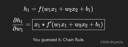
你猜对了，链式法则。You guessed it, Chain Rule.

这里的 x1 是体重，x2 是身高。这是我们第二次看到 f'(x)（Sigmoid 函数的导数）！让我们推导一下：
x1​ here is weight, and x2 is height. This is the second time we’ve seen f′(x) (the derivate of the sigmoid function) now! Let’s derive it:

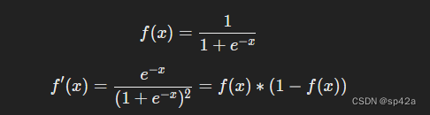
稍后我们会使用这个简洁的形式的 f′(x)。
We’ll use this nice form for f′(x) later.

我们完成了！我们已经成功将 ∂L/∂w1 分解成了几个我们可以计算的部分：
We’re done! We’ve managed to break down∂L/∂w1into several parts we can calculate:

这种通过反向传播计算偏导数的系统被称为反向传播，或简称为“反播”。
This system of calculating partial derivatives by working backwards is known as backpropagation, or “backprop”.

哦，那是很多符号 - 如果你仍然有点困惑，没关系。让我们做一个例子来看看它是如何运作的！
Phew. That was a lot of symbols - it’s alright if you’re still a bit confused. Let’s do an example to see this in action!

例子：计算偏导数 Example: Calculating the Partial Derivative

我们将继续假设我们的数据集中只有 Alice：
We’re going to continue pretending only Alice is in our dataset:

让我们将所有权重初始化 1，所有偏置初始化为 0。如果我们通过网络进行前向传播，我们会得到：
Let’s initialize all the weights to 1 and all the biases to 0. If we do a feedforward pass through the network, we get:

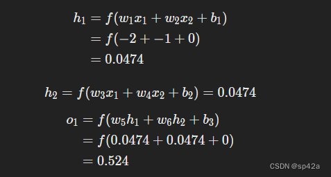
网络输出ypred=0.524，这并不明显偏向于男性（0）或女性（1）。让我们计算∂L/∂w_1：
The network outputs ypred=0.524, which doesn’t strongly favor Male (0) or Female (1). Let’s calculate ∂L/∂w1​:

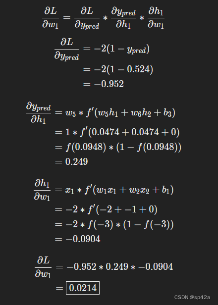
提醒：我们之前推导出了对于 Sigmoid 激活函数的导数公式为 f'(x) = f(x) * (1 - f(x))。
Reminder: we derived f′(x)=f(x)∗(1−f(x)) for our sigmoid activation function earlier.

我们做到了！这告诉我们，如果我们增加 w_1，损失函数 L 会因此稍微增加一点点。
We did it! This tells us that if we were to increase w1​, L would increase a tiiiny bit as a result.

训练：随机梯度下降 Training: Stochastic Gradient Descent

我们现在拥有所有训练神经网络所需的工具！ 我们将使用一种名为随机梯度下降（SGD）的优化算法，它告诉我们如何调整权重和偏置以最小化损失。其基本更新方程如下：
We have all the tools we need to train a neural network now! We’ll use an optimization algorithm called stochastic gradient descent (SGD) that tells us how to change our weights and biases to minimize loss. It’s basically just this update equation:

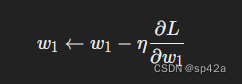
其中，η 是一个称为学习率的常数，控制着训练的速度。我们所做的就是从 w1 中减去 η(∂L/∂w1)：
η is a constant called the learning rate that controls how fast we train. All we’re doing is subtracting η(∂L/∂w1) from w1​:

• 如果 ∂L/∂w1 是正数，w1 将减小，从而使损失 L 减小。If ∂L∂w1∂w1​∂L​ is positive, w1w1​ will decrease, which makes L decrease.
• 如果 ∂L/∂w1 是负数，w1 将增加，从而使损失 L 减小。If ∂L∂w1∂w1​∂L​ is negative, w1w1​ will increase, which makes L decrease.

如果我们对网络中的每个权重和偏差都这样操作，损失将逐渐减小，我们的网络将得到改进。
If we do this for every weight and bias in the network, the loss will slowly decrease and our network will improve.

我们的训练过程将如下所示：Our training process will look like this:

1. 从数据集中选择一个样本。这就是所谓的随机梯度下降 - 我们一次只操作一个样本。Choose one sample from our dataset. This is what makes it stochastic gradient descent - we only operate on one sample at a time.
2. 计算损失对权重或偏差的所有偏导数，例如 ∂L/∂w1、∂L/∂w2 Calculate all the partial derivatives of loss with respect to weights or biases
3. 使用更新方程更新每个权重和偏差 Use the update equation to update each weight and bias.
4. 返回到步骤 1Go back to step 1.

我们看看它是如何运作的！Let’s see it in action!

代码：一个完整的神经网络 Code: A Complete Neural Network

最后实现一个完整的神经网络：
It’s finally time to implement a complete neural network:

import numpy as np

def sigmoid(x):
  # Sigmoid activation function: f(x) = 1 / (1 + e^(-x))
  return 1 / (1 + np.exp(-x))

def deriv_sigmoid(x):
  # Derivative of sigmoid: f'(x) = f(x) * (1 - f(x))
  fx = sigmoid(x)
  return fx * (1 - fx)

def mse_loss(y_true, y_pred):
  # y_true and y_pred are numpy arrays of the same length.
  return ((y_true - y_pred) ** 2).mean()

class OurNeuralNetwork:
  '''
  A neural network with:
    - 2 inputs
    - a hidden layer with 2 neurons (h1, h2)
    - an output layer with 1 neuron (o1)

  *** DISCLAIMER ***:
  The code below is intended to be simple and educational, NOT optimal.
  Real neural net code looks nothing like this. DO NOT use this code.
  Instead, read/run it to understand how this specific network works.
  '''
  def __init__(self):
    # Weights
    self.w1 = np.random.normal()
    self.w2 = np.random.normal()
    self.w3 = np.random.normal()
    self.w4 = np.random.normal()
    self.w5 = np.random.normal()
    self.w6 = np.random.normal()

    # Biases
    self.b1 = np.random.normal()
    self.b2 = np.random.normal()
    self.b3 = np.random.normal()

  def feedforward(self, x):
    # x is a numpy array with 2 elements.
    h1 = sigmoid(self.w1 * x[0] + self.w2 * x[1] + self.b1)
    h2 = sigmoid(self.w3 * x[0] + self.w4 * x[1] + self.b2)
    o1 = sigmoid(self.w5 * h1 + self.w6 * h2 + self.b3)
    return o1

  def train(self, data, all_y_trues):
    '''
    - data is a (n x 2) numpy array, n = # of samples in the dataset.
    - all_y_trues is a numpy array with n elements.
      Elements in all_y_trues correspond to those in data.
    '''
    learn_rate = 0.1
    epochs = 1000 # 遍历整个数据集的次数 number of times to loop through the entire dataset

    for epoch in range(epochs):
      for x, y_true in zip(data, all_y_trues):
        # --- Do a feedforward (we'll need these values later)
        sum_h1 = self.w1 * x[0] + self.w2 * x[1] + self.b1
        h1 = sigmoid(sum_h1)

        sum_h2 = self.w3 * x[0] + self.w4 * x[1] + self.b2
        h2 = sigmoid(sum_h2)

        sum_o1 = self.w5 * h1 + self.w6 * h2 + self.b3
        o1 = sigmoid(sum_o1)
        y_pred = o1

        # --- 计算偏导数 Calculate partial derivatives.
        # --- Naming: d_L_d_w1 represents "partial L / partial w1"
        d_L_d_ypred = -2 * (y_true - y_pred)

        # Neuron o1
        d_ypred_d_w5 = h1 * deriv_sigmoid(sum_o1)
        d_ypred_d_w6 = h2 * deriv_sigmoid(sum_o1)
        d_ypred_d_b3 = deriv_sigmoid(sum_o1)

        d_ypred_d_h1 = self.w5 * deriv_sigmoid(sum_o1)
        d_ypred_d_h2 = self.w6 * deriv_sigmoid(sum_o1)

        # Neuron h1
        d_h1_d_w1 = x[0] * deriv_sigmoid(sum_h1)
        d_h1_d_w2 = x[1] * deriv_sigmoid(sum_h1)
        d_h1_d_b1 = deriv_sigmoid(sum_h1)

        # Neuron h2
        d_h2_d_w3 = x[0] * deriv_sigmoid(sum_h2)
        d_h2_d_w4 = x[1] * deriv_sigmoid(sum_h2)
        d_h2_d_b2 = deriv_sigmoid(sum_h2)

        # --- 更新权重偏差 Update weights and biases
        # Neuron h1
        self.w1 -= learn_rate * d_L_d_ypred * d_ypred_d_h1 * d_h1_d_w1
        self.w2 -= learn_rate * d_L_d_ypred * d_ypred_d_h1 * d_h1_d_w2
        self.b1 -= learn_rate * d_L_d_ypred * d_ypred_d_h1 * d_h1_d_b1

        # Neuron h2
        self.w3 -= learn_rate * d_L_d_ypred * d_ypred_d_h2 * d_h2_d_w3
        self.w4 -= learn_rate * d_L_d_ypred * d_ypred_d_h2 * d_h2_d_w4
        self.b2 -= learn_rate * d_L_d_ypred * d_ypred_d_h2 * d_h2_d_b2

        # Neuron o1
        self.w5 -= learn_rate * d_L_d_ypred * d_ypred_d_w5
        self.w6 -= learn_rate * d_L_d_ypred * d_ypred_d_w6
        self.b3 -= learn_rate * d_L_d_ypred * d_ypred_d_b3

      # --- 在每个时代结束时计算总损失 Calculate total loss at the end of each epoch
      if epoch % 10 == 0:
        y_preds = np.apply_along_axis(self.feedforward, 1, data)
        loss = mse_loss(all_y_trues, y_preds)
        print("Epoch %d loss: %.3f" % (epoch, loss))

# 定义数据集 Define dataset
data = np.array([
  [-2, -1],  # Alice
  [25, 6],   # Bob
  [17, 4],   # Charlie
  [-15, -6], # Diana
])
all_y_trues = np.array([
  1, # Alice
  0, # Bob
  0, # Charlie
  1, # Diana
])

# 训练我们的神经网络 Train our neural network!
network = OurNeuralNetwork()
network.train(data, all_y_trues)

You can run / play with this code yourself. It’s also available on Github.

我们的损失持续下降，表示网络正在学习中。Our loss steadily decreases as the network learns:

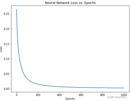
现在我们可以用该网络预测性别：
We can now use the network to predict genders:

# 进行预测 Make some predictions
emily = np.array([-7, -3]) # 128 pounds, 63 inches
frank = np.array([20, 2])  # 155 pounds, 68 inches
print("Emily: %.3f" % network.feedforward(emily)) # 0.951 - F
print("Frank: %.3f" % network.feedforward(frank)) # 0.039 - M