


之前提到过聚类之后,聚类质量的评价:
聚类︱python实现 六大 分群质量评估指标(兰德系数、互信息、轮廓系数)
R语言相关分类效果评估:
R语言︱分类器的性能表现评价(混淆矩阵,准确率,召回率,F1,mAP、ROC曲线)
.
文章目录
- 一、acc、recall、F1、混淆矩阵、分类综合报告
- 二、ROC
- 三、距离
- 四、回归
- 五 合理的进行绘图(混淆矩阵/ROC)
一、acc、recall、F1、混淆矩阵、分类综合报告
1、准确率
第一种方式:accuracy_score
# 准确率
import numpy as np
from sklearn.metrics import accuracy_score
y_pred = [0, 2, 1, 3,9,9,8,5,8]
y_true = [0, 1, 2, 3,2,6,3,5,9]
accuracy_score(y_true, y_pred)
Out[127]: 0.33333333333333331
accuracy_score(y_true, y_pred, normalize=False) # 类似海明距离,每个类别求准确后,再求微平均
Out[128]: 3
- 1
- 2
- 3
- 4
- 5
- 6
- 7
- 8
- 9
- 10
- 11
第二种方式:metrics
宏平均比微平均更合理,但也不是说微平均一无是处,具体使用哪种评测机制,还是要取决于数据集中样本分布
宏平均(Macro-averaging),是先对每一个类统计指标值,然后在对所有类求算术平均值。
微平均(Micro-averaging),是对数据集中的每一个实例不分类别进行统计建立全局混淆矩阵,然后计算相应指标。(来源:谈谈评价指标中的宏平均和微平均)
from sklearn import metrics
metrics.precision_score(y_true, y_pred, average='micro')  # 微平均,精确率
Out[130]: 0.33333333333333331
metrics.precision_score(y_true, y_pred, average=‘macro’) # 宏平均,精确率
Out[131]: 0.375
metrics.precision_score(y_true, y_pred, labels=[0, 1, 2, 3], average=‘macro’) # 指定特定分类标签的精确率
Out[133]: 0.5
- 1
- 2
- 3
- 4
- 5
- 6
- 7
- 8
- 9
2_52" target="_blank">其中average参数有五种:(None, ‘micro’, ‘macro’, ‘weighted’, ‘samples’)
.
2、召回率
metrics.recall_score(y_true, y_pred, average='micro')
Out[134]: 0.33333333333333331

metrics.recall_score(y_true, y_pred, average='macro')
Out[135]: 0.3125
- 1
- 2
- 3
- 4
- 5
.
3、F1
metrics.f1_score(y_true, y_pred, average='weighted')
Out[136]: 0.37037037037037035
- 1
- 2
- 3
.
4、混淆矩阵
# 混淆矩阵
from sklearn.metrics import confusion_matrix
confusion_matrix(y_true, y_pred)
Out[137]:
array([[1, 0, 0, …, 0, 0, 0],
[0, 0, 1, …, 0, 0, 0],
[0, 1, 0, …, 0, 0, 1],
…,
[0, 0, 0, …, 0, 0, 1],
[0, 0, 0, …, 0, 0, 0],
[0, 0, 0, …, 0, 1, 0]])
- 1
- 2
- 3
- 4
- 5
- 6
- 7
- 8
- 9
- 10
- 11
- 12
5__91" target="_blank">横为true label 竖为predict

.
5、 分类报告
# 分类报告:precision/recall/fi-score/均值/分类个数
 from sklearn.metrics import classification_report
 y_true = [0, 1, 2, 2, 0]
 y_pred = [0, 0, 2, 2, 0]
 target_names = ['class 0', 'class 1', 'class 2']
 print(classification_report(y_true, y_pred, target_names=target_names))
- 1
- 2
- 3
- 4
- 5
- 6
其中的结果:
precision recall f1-score supportclass 0 0.67 1.00 0.80 2 class 1 0.00 0.00 0.00 1 class 2 1.00 1.00 1.00 2
avg / total 0.67 0.80 0.72 5
- 1
- 2
- 3
- 4
- 5
- 6
- 7
6_kappa_score_115" target="_blank">包含:precision/recall/fi-score/均值/分类个数
.
6、 kappa score
kappa score是一个介于(-1, 1)之间的数. score>0.8意味着好的分类;0或更低意味着不好(实际是随机标签)
 from sklearn.metrics import cohen_kappa_score
 y_true = [2, 0, 2, 2, 0, 1]
 y_pred = [0, 0, 2, 2, 0, 2]
 cohen_kappa_score(y_true, y_pred)
- 1
- 2
- 3
- 4
.
二、ROC
1、计算ROC值
import numpy as np
 from sklearn.metrics import roc_auc_score
 y_true = np.array([0, 0, 1, 1])
 y_scores = np.array([0.1, 0.4, 0.35, 0.8])
 roc_auc_score(y_true, y_scores)
- 1
- 2
- 3
- 4
- 5
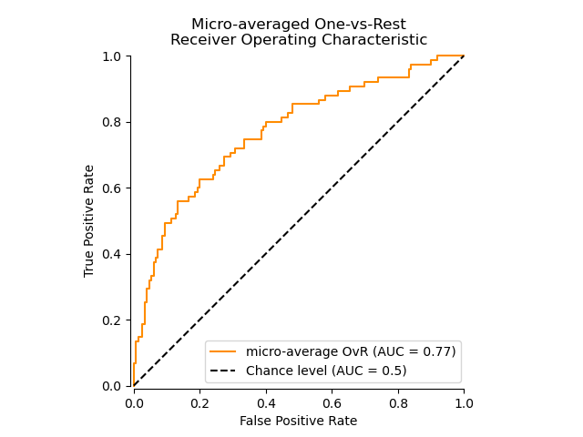
2、ROC曲线
 y = np.array([1, 1, 2, 2])
 scores = np.array([0.1, 0.4, 0.35, 0.8])
 fpr, tpr, thresholds = roc_curve(y, scores, pos_label=2)
- 1
- 2
- 3
来看一个官网例子,贴部分代码,全部的code见:Receiver Operating Characteristic (ROC)
import numpy as np
import matplotlib.pyplot as plt
from itertools import cycle
from sklearn import svm, datasets
from sklearn.metrics import roc_curve, auc
from sklearn.model_selection import train_test_split
from sklearn.preprocessing import label_binarize
from sklearn.multiclass import OneVsRestClassifier
from scipy import interp
Import some data to play with
iris = datasets.load_iris()
X = iris.data
y = iris.target
画图
all_fpr = np.unique(np.concatenate([fpr[i] for i in range(n_classes)]))
Then interpolate all ROC curves at this points
mean_tpr = np.zeros_like(all_fpr)
for i in range(n_classes):
mean_tpr += interp(all_fpr, fpr[i], tpr[i])
Finally average it and compute AUC
mean_tpr /= n_classes
fpr[“macro”] = all_fpr
tpr[“macro”] = mean_tpr
roc_auc[“macro”] = auc(fpr[“macro”], tpr[“macro”])
Plot all ROC curves
plt.figure()
plt.plot(fpr[“micro”], tpr[“micro”],
label=‘micro-average ROC curve (area = {0:0.2f})’
‘’.format(roc_auc[“micro”]),
color=‘deeppink’, linestyle=’:’, linewidth=4)
plt.plot(fpr[“macro”], tpr[“macro”],
label=‘macro-average ROC curve (area = {0:0.2f})’
‘’.format(roc_auc[“macro”]),
color=‘navy’, linestyle=’:’, linewidth=4)
colors = cycle([‘aqua’, ‘darkorange’, ‘cornflowerblue’])
for i, color in zip(range(n_classes), colors):
plt.plot(fpr[i], tpr[i], color=color, lw=lw,
label=‘ROC curve of class {0} (area = {1:0.2f})’
‘’.format(i, roc_auc[i]))
plt.plot([0, 1], [0, 1], ‘k–’, lw=lw)
plt.xlim([0.0, 1.0])
plt.ylim([0.0, 1.05])
plt.xlabel(‘False Positive Rate’)
plt.ylabel(‘True Positive Rate’)
plt.title(‘Some extension of Receiver operating characteristic to multi-class’)
plt.legend(loc=“lower right”)
plt.show()
- 1
- 2
- 3
- 4
- 5
- 6
- 7
- 8
- 9
- 10
- 11
- 12
- 13
- 14
- 15
- 16
- 17
- 18
- 19
- 20
- 21
- 22
- 23
- 24
- 25
- 26
- 27
- 28
- 29
- 30
- 31
- 32
- 33
- 34
- 35
- 36
- 37
- 38
- 39
- 40
- 41
- 42
- 43
- 44
- 45
- 46
- 47
- 48
- 49
- 50
- 51
- 52
- 53
- 54
- 55
- 56
- 57
- 58
.
三、距离
.
1、海明距离
from sklearn.metrics import hamming_loss
 y_pred = [1, 2, 3, 4]
 y_true = [2, 2, 3, 4]
 hamming_loss(y_true, y_pred)
0.25
- 1
- 2
- 3
- 4
- 5
.
2、Jaccard距离
 import numpy as np
 from sklearn.metrics import jaccard_similarity_score
 y_pred = [0, 2, 1, 3,4]
 y_true = [0, 1, 2, 3,4]
 jaccard_similarity_score(y_true, y_pred)
0.5
 jaccard_similarity_score(y_true, y_pred, normalize=False)
2
- 1
- 2
- 3
- 4
- 5
- 6
- 7
- 8
.
四、回归
1、 可释方差值(Explained variance score)
 from sklearn.metrics import explained_variance_score
y_true = [3, -0.5, 2, 7]
 y_pred = [2.5, 0.0, 2, 8]
 explained_variance_score(y_true, y_pred)
- 1
- 2
- 3
- 4
.
2、 平均绝对误差(Mean absolute error)
from sklearn.metrics import mean_absolute_error
 y_true = [3, -0.5, 2, 7]
 y_pred = [2.5, 0.0, 2, 8]
 mean_absolute_error(y_true, y_pred)
- 1
- 2
- 3
- 4
.
3、 均方误差(Mean squared error)
 from sklearn.metrics import mean_squared_error
 y_true = [3, -0.5, 2, 7]
 y_pred = [2.5, 0.0, 2, 8]
 mean_squared_error(y_true, y_pred)
- 1
- 2
- 3
- 4
.
4、中值绝对误差(Median absolute error)
 from sklearn.metrics import median_absolute_error
 y_true = [3, -0.5, 2, 7]
 y_pred = [2.5, 0.0, 2, 8]
 median_absolute_error(y_true, y_pred)
- 1
- 2
- 3
- 4
.
5、 R方值,确定系数
 from sklearn.metrics import r2_score
 y_true = [3, -0.5, 2, 7]
 y_pred = [2.5, 0.0, 2, 8]
 r2_score(y_true, y_pred)
- 1
- 2
- 3
- 4
.
五 合理的进行绘图(混淆矩阵/ROC)
%matplotlib inline
import itertools
import numpy as np
import matplotlib.pyplot as plt
from sklearn import svm, datasets
from sklearn.model_selection import train_test_split
from sklearn.metrics import f1_score,accuracy_score,recall_score,classification_report,confusion_matrix
def plot_confusion_matrix(cm, classes,
normalize=False,
title=‘Confusion matrix’,
cmap=plt.cm.Blues):
“”"
This function prints and plots the confusion matrix.
Normalization can be applied by setting normalize=True.
“”"
if normalize:
cm = cm.astype(‘float’) / cm.sum(axis=1)[:, np.newaxis]
print(“Normalized confusion matrix”)
else:
print(‘Confusion matrix, without normalization’)
print(cm)

plt.imshow(cm, interpolation='nearest', cmap=cmap)
plt.title(title)
plt.colorbar()
tick_marks = np.arange(len(classes))
plt.xticks(tick_marks, classes, rotation=45)
plt.yticks(tick_marks, classes)

fmt = '.2f' if normalize else 'd'
thresh = cm.max() / 2.
for i, j in itertools.product(range(cm.shape[0]), range(cm.shape[1])):
    plt.text(j, i, format(cm[i, j], fmt),
             horizontalalignment="center",
             color="white" if cm[i, j] > thresh else "black")

plt.tight_layout()
plt.ylabel('True label')
plt.xlabel('Predicted label')
def CalculationResults(val_y,y_val_pred,simple = False,
target_names = [‘class_-2_Not_mentioned’,‘class_-1_Negative’,‘class_0_Neutral’,‘class_1_Positive’]):
# 计算检验
F1_score = f1_score(val_y,y_val_pred, average=‘macro’)
if simple:
return F1_score
else:
acc = accuracy_score(val_y,y_val_pred)
recall_score_ = recall_score(val_y,y_val_pred, average=‘macro’)
confusion_matrix_ = confusion_matrix(val_y,y_val_pred)
class_report = classification_report(val_y, y_val_pred, target_names=target_names)
print(‘f1_score:’,F1_score,‘ACC_score:’,acc,‘recall:’,recall_score_)
print(’\n----class report —:\n’,class_report)
#print(’----confusion matrix —:\n’,confusion_matrix_)
    # 画混淆矩阵
        # 画混淆矩阵图
    plt.figure()
    plot_confusion_matrix(confusion_matrix_, classes=target_names,
                          title='Confusion matrix, without normalization')
    plt.show()
    return F1_score,acc,recall_score_,confusion_matrix_,class_report
- 1
- 2
- 3
- 4
- 5
- 6
- 7
- 8
- 9
- 10
- 11
- 12
- 13
- 14
- 15
- 16
- 17
- 18
- 19
- 20
- 21
- 22
- 23
- 24
- 25
- 26
- 27
- 28
- 29
- 30
- 31
- 32
- 33
- 34
- 35
- 36
- 37
- 38
- 39
- 40
- 41
- 42
- 43
- 44
- 45
- 46
- 47
- 48
- 49
- 50
- 51
- 52
- 53
- 54
- 55
- 56
- 57
- 58
- 59
- 60
- 61
- 62
- 63
- 64
- 65
- 66
函数plot_confusion_matrix是绘制混淆矩阵的函数,CalculationResults则为只要给入y的预测值 + 实际值,以及分类的标签大致内容,就可以一次性输出:f1值,acc,recall以及报表
输出结果的部分,如下:
f1_score: 0.6111193724134587 ACC_score: 0.9414 recall: 0.5941485524896096
----class report —:
precision recall f1-score support
class_-2_Not_mentioned 0.96 0.97 0.97 11757
class_-1_Negative 0.68 0.51 0.58 182
class_0_Neutral 1.00 0.01 0.01 136
class_1_Positive 0.87 0.89 0.88 2925
avg / total 0.94 0.94 0.94 15000
Confusion matrix, without normalization
[[11437 27 0 293]
[ 72 93 0 17]
[ 63 10 1 62]
[ 328 7 0 2590]]
- 1
- 2
- 3
- 4
- 5
- 6
- 7
- 8
- 9
- 10
- 11
- 12
- 13
- 14
- 15
- 16
- 17
参考文献:
        </div>
					<link href="https://csdnimg.cn/release/phoenix/mdeditor/markdown_views-7b4cdcb592.css" rel="stylesheet">
            </div>


 1万+
1万+


 被折叠的 条评论
为什么被折叠?
被折叠的 条评论
为什么被折叠?
 到【灌水乐园】发言


