如何用Tensorflow实现增强版本的Mnist手写识别网络模型

上一个阶段构造的简单模型训练后，只有91%正确率。本文章讲解如何用一个稍微复杂的模型：卷积神经网络来提升效果。
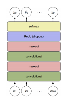
下面是效果图：

图1

具体的步骤为：

首先完成准备工作：

import input_data
import tensorflow as tf
#导入数据
mnist = input_data.read_data_sets('MNIST_data', one_hot = True)
#设置占位符和输入数据的格式
x = tf.placeholder("float", shape = [None, 784])
y = tf.placeholder("float' shape = [None, 10])

#784=>>28*28, 最后一维代表图片的颜色通道数,这里是灰度图为1,如果是rgb彩色图，则为3.
x_image = tf.reshape(x, [-1,28,28,1]) #

定义权重初始化函数

在初始化W和b时应该加入少量的噪声来打破对称性以及避免0梯度。为了不在建立模型的时候反复做初始化操作，定义两个函数用于初始化：

#其实现在的W就是卷积核（filters），是不断学习的参数
def weight_variable(shape):
    initial = tf.truncated_normal(shape, stddev = 0.1) # 从正态分布中取样，stddev表示标准差
    return tf.Variable(initial)

def bias_variable(shaple):
    initial = tf.constant(0.1, shape = shape)
    return tf.Variable(initial)

定义卷积和池化函数

def conv2d(x, W):
    #x是输入，W是卷积核filter，[1,1,1,1]分别对应着输入数据的4个维度[batch, height, width, channels],在这里使用1步长（stride size），‘SAME’代表0边距（padding size）卷积过程超出图片的范围，用0代替。保证卷积后map大小和输入一样。
    return tf.nn.conv2d(x, W, strides=[1,1,1,1], padding = 'SAME')

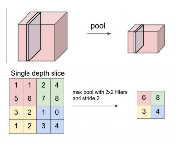
def max_pool_2x2(x):
    #x是输入；ksize[1,2,2,1]对应着输入数据的4个维度，长度>=4；strides对应输入数据4个维度，长度>=4；‘SAME’代表0边距（padding size）
    return tf.nn.max_pool(x, ksize = [1,2,2,1], strides = [1,2,2,1], padding = 'SAME')

其中max pooling操作图为：

图2

实现第一层卷积

如图1所示，由一个卷积接一个max pooling完成。

#卷积的权重张量形状是[5, 5, 1, 32]，前两维度代表patch的大小为5*5，接着是输入的通道数目，最后是输出的通道数目。便于理解：输入的通道数相当于上一层的map数，输出的通道数目就是卷积核的个数，也就是下一层的map数。
W_conv1 = weight_variable([5,5,1,32]) 
#每一个输出通道都有一个对应的偏置量
b_conv1 = bias_variable([32])

#把x_image和权值向量进行卷积，加上偏置项，然后应用ReLU激活函数，
h_conv1 = tf.nn.relu(conv2d(x_image,W_conv1) + b_conv1) #1*28*28 ==> 28*28*32
#进行max pooling
h_pool1 = max_pool_2x2(h_conv1) # 32*24*24 ==> 14*14*32

实现第二层卷积

W_conv2 = weight_variable([5,5,32,64]) 
b_conv2 = bias_variable([64])
h_conv2 = tf.nn.relu(conv2d(h_pool1, W_conv2) + b_conv2) #32*14*14 ⇒ 14*14*64
h_pool2 = max_pool_2x2(h_conv2) #64*14*14 ==> 7*7*64

密集连接层

图片尺寸减小到7x7后，加入一个有1024个神经元的全连接层，用于处理整个图片。

W_fc1 = weight_variable([7*7*64, 1024]) #转换成flat vector
b_fc1 = bias_variable([1024])

h_pool2_flat = tf.reshape(h_pool2, [-1, 7*7*64]) #将上一层的输出也转换成flat vector
h_fc1 = tf.nn.relu(tf.matmul(h_pool2_flat, W_fc1) + b_fc1) #relu（W*x+b）的形式

加入dropout，防止过拟合

keep_prob = tf.placeholder("float") #用一个placeholder来代表一个神经元的输出在dropout中保持不变的概率.在训练过程中启用dropout，在测试过程中关闭dropout
h_fc1_drop = tf.nn.dropout(h_fc1, keep_prob)

输出层

W_fc2 = weight_variable([1024, 10])
b_fc2 = bias_variable([10])
#添加一个softmax层
y_conv = tf.nn.softmax(tf.matmul(h_fc1_drop, W_fc2) + b_fc2)

训练和评估模型

cross_entropy = -tf.reduce_sum(y_*tf.log(y_conv)) #定义loss函数
train_step = tf.train.AdamOptimizer(le-4).minimize(cross_entropy) #定义训练算法，这里使用更加复杂的ADAM优化器
sess = tf.InteractiveSession() #开始一个会话
sess.run(tf.initialize_all_variables()) # 初始化变量
#在训练之前定义准确预测操作
correct_prediction = tf.equal(tf.argmax(y_conv1, 1), tf.argmax(y_, 1))
accuracy = tf.reduce_mean(tf.cast(correct_prediction, "float"))

#训练模型
for n in range(20000):
    batch = mnist.train.next_batch(50)
    if n%100 == 0:
        train_accuracy = accuracy.eval(feed_dict = {x:batch[0],y:batch[1],keep_prob: 1.0})
        print "step %d, training accuracy %g" %(n, train_accuracy)
    sess.run(train_step, feed_dict = {x:batch[0], y:batch[1], keep_prob: 0.5})

#评估准确率
print "test accuracy %g" %accuracy.eval(feed_dict = {x:mnist.test.image, y:mnist.test.labels, keep_prob: 1.0})

以上代码，在最终测试集上的准确率大概是99.2%。