【NLP】DSSM深度结构化语义模型原理

DSSM

Deep Structured Semantic Model

DSSM的结构

Learning Deep Structured Semantic Models for Web Search using Clickthrough Data以及其后续文章

A Multi-View Deep Learning Approach for Cross Domain User Modeling in Recommendation Systems的实现Demo。

1. 数据

DSSM，对于输入数据是Query对，即Query短句和相应的展示，展示中分点击和未点击，分别为正负样，同时对于点击的先后顺序，也是有不同赋值，具体可参考论文。

对于我的Query数据本人无权开放，还请自行寻找数据。

2. word hashing

原文使用3-grams，对于中文，我使用了uni-gram，因为中文本身字有一定代表意义（也有论文拆笔画），对于每个gram都使用one-hot编码代替，最终可以大大降低短句维度。

3. 结构

结构图：

1. 把条目映射成低维向量。
2. 计算查询和文档的cosine相似度。

3.1 输入

这里使用了TensorBoard可视化，所以定义了name_scope:

with tf.name_scope('input'):
    query_batch = tf.sparse_placeholder(tf.float32, shape=[None, TRIGRAM_D], name='QueryBatch')
    doc_positive_batch = tf.sparse_placeholder(tf.float32, shape=[None, TRIGRAM_D], name='DocBatch')
    doc_negative_batch = tf.sparse_placeholder(tf.float32, shape=[None, TRIGRAM_D], name='DocBatch')
    on_train = tf.placeholder(tf.bool)
   
   
1
2
3
4
5

3.2 全连接层

我使用三层的全连接层，对于每一层全连接层，除了神经元不一样，其他都一样，所以可以写一个函数复用。 

ln=Wnx+b1 ln=Wnx+b1

def add_layer(inputs, in_size, out_size, activation_function=None):
    wlimit = np.sqrt(6.0 / (in_size + out_size))
    Weights = tf.Variable(tf.random_uniform([in_size, out_size], -wlimit, wlimit))
    biases = tf.Variable(tf.random_uniform([out_size], -wlimit, wlimit))
    Wx_plus_b = tf.matmul(inputs, Weights) + biases
    if activation_function is None:
        outputs = Wx_plus_b
    else:
        outputs = activation_function(Wx_plus_b)
    return outputs
   
   
1
2
3
4
5
6
7
8
9
10

其中，对于权重和Bias，使用了按照论文的特定的初始化方式：

    wlimit = np.sqrt(6.0 / (in_size + out_size))
    Weights = tf.Variable(tf.random_uniform([in_size, out_size], -wlimit, wlimit))
    biases = tf.Variable(tf.random_uniform([out_size], -wlimit, wlimit))
   
   
1
2
3

Batch Normalization

def batch_normalization(x, phase_train, out_size):
    """
    Batch normalization on convolutional maps.
    Ref.: http://stackoverflow.com/questions/33949786/how-could-i-use-batch-normalization-in-tensorflow
    Args:
        x:           Tensor, 4D BHWD input maps
        out_size:       integer, depth of input maps
        phase_train: boolean tf.Varialbe, true indicates training phase
        scope:       string, variable scope
    Return:
        normed:      batch-normalized maps
    """
    with tf.variable_scope('bn'):
        beta = tf.Variable(tf.constant(0.0, shape=[out_size]),
                           name='beta', trainable=True)
        gamma = tf.Variable(tf.constant(1.0, shape=[out_size]),
                            name='gamma', trainable=True)
        batch_mean, batch_var = tf.nn.moments(x, [0], name='moments')
        ema = tf.train.ExponentialMovingAverage(decay=0.5)

        def mean_var_with_update():
            ema_apply_op = ema.apply([batch_mean, batch_var])
            with tf.control_dependencies([ema_apply_op]):
                return tf.identity(batch_mean), tf.identity(batch_var)

        mean, var = tf.cond(phase_train,
                            mean_var_with_update,
                            lambda: (ema.average(batch_mean), ema.average(batch_var)))
        normed = tf.nn.batch_normalization(x, mean, var, beta, gamma, 1e-3)
    return normed
   
   
1
2
3
4
5
6
7
8
9
10
11
12
13
14
15
16
17
18
19
20
21
22
23
24
25
26
27
28
29
30

单层

with tf.name_scope('FC1'):
    # 激活函数在BN之后，所以此处为None
    query_l1 = add_layer(query_batch, TRIGRAM_D, L1_N, activation_function=None)
    doc_positive_l1 = add_layer(doc_positive_batch, TRIGRAM_D, L1_N, activation_function=None)
    doc_negative_l1 = add_layer(doc_negative_batch, TRIGRAM_D, L1_N, activation_function=None)

with tf.name_scope('BN1'):
    query_l1 = batch_normalization(query_l1, on_train, L1_N)
    doc_l1 = batch_normalization(tf.concat([doc_positive_l1, doc_negative_l1], axis=0), on_train, L1_N)
    doc_positive_l1 = tf.slice(doc_l1, [0, 0], [query_BS, -1])
    doc_negative_l1 = tf.slice(doc_l1, [query_BS, 0], [-1, -1])
    query_l1_out = tf.nn.relu(query_l1)
    doc_positive_l1_out = tf.nn.relu(doc_positive_l1)
    doc_negative_l1_out = tf.nn.relu(doc_negative_l1)
······
   
   
1
2
3
4
5
6
7
8
9
10
11
12
13
14
15

合并负样本

with tf.name_scope('Merge_Negative_Doc'):
    # 合并负样本，tile可选择是否扩展负样本。
    doc_y = tf.tile(doc_positive_y, [1, 1])
    for i in range(NEG):
        for j in range(query_BS):
            # slice(input_, begin, size)切片API
            doc_y = tf.concat([doc_y, tf.slice(doc_negative_y, [j * NEG + i, 0], [1, -1])], 0)
   
   
1
2
3
4
5
6
7

3.3 计算cos相似度

with tf.name_scope('Cosine_Similarity'):
    # Cosine similarity
    # query_norm = sqrt(sum(each x^2))
    query_norm = tf.tile(tf.sqrt(tf.reduce_sum(tf.square(query_y), 1, True)), [NEG + 1, 1])
    # doc_norm = sqrt(sum(each x^2))
    doc_norm = tf.sqrt(tf.reduce_sum(tf.square(doc_y), 1, True))

    prod = tf.reduce_sum(tf.multiply(tf.tile(query_y, [NEG + 1, 1]), doc_y), 1, True)
    norm_prod = tf.multiply(query_norm, doc_norm)

    # cos_sim_raw = query * doc / (||query|| * ||doc||)
    cos_sim_raw = tf.truediv(prod, norm_prod)
    # gamma = 20
    cos_sim = tf.transpose(tf.reshape(tf.transpose(cos_sim_raw), [NEG + 1, query_BS])) * 20
   
   
1
2
3
4
5
6
7
8
9
10
11
12
13
14

3.4 定义损失函数

with tf.name_scope('Loss'):
    # Train Loss
    # 转化为softmax概率矩阵。
    prob = tf.nn.softmax(cos_sim)
    # 只取第一列，即正样本列概率。
    hit_prob = tf.slice(prob, [0, 0], [-1, 1])
    loss = -tf.reduce_sum(tf.log(hit_prob))
    tf.summary.scalar('loss', loss)
   
   
1
2
3
4
5
6
7
8

3.5选择优化方法

with tf.name_scope('Training'):
    # Optimizer
    train_step = tf.train.AdamOptimizer(FLAGS.learning_rate).minimize(loss)
   
   
1
2
3

## 3.6 开始训练

# 创建一个Saver对象，选择性保存变量或者模型。
saver = tf.train.Saver()
# with tf.Session(config=config) as sess:
with tf.Session() as sess:
    sess.run(tf.global_variables_initializer())
    train_writer = tf.summary.FileWriter(FLAGS.summaries_dir + '/train', sess.graph)
    start = time.time()
    for step in range(FLAGS.max_steps):
        batch_id = step % FLAGS.epoch_steps
        sess.run(train_step, feed_dict=feed_dict(True, True, batch_id % FLAGS.pack_size, 0.5))
   
   
1
2
3
4
5
6
7
8
9
10

GitHub完整代码 https://github.com/InsaneLife/dssm

Multi-view DSSM实现同理，可以参考GitHub：multi_view_dssm_v3

CSDN原文：http://blog.csdn.net/shine19930820/article/details/79042567

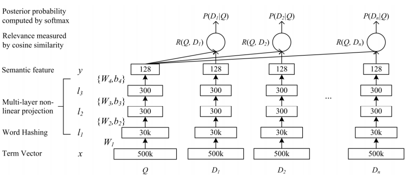
版权声明：本文为博主原创文章，转载请注明出处：http://blog.csdn.net/shine19930820 https://blog.csdn.net/shine19930820/article/details/79042567

上面是 DSSM 训练的架构图:

1. 输入的是一个 query 和这个query相关的 doc ，这里的输入特征可以是最简单的 one-hot ,而需要 train 的是这个query下各个doc的相关性( DSSM 里面使用点击率来代替相关性)

2. 由于这种 one-hot 的输入可能会有两个问题:

   1. 导致 vocabulary 太大

   2. 会出现 oov 的问题

      因此输入特征之后的第一层是做一个叫做 Word Hashinging 的操作

3. 接下来就是传统的神经网络了 
   $$l_i=f(W_il_{i-1}+b_i),i = 2,…,N-1 \\ 
   y=f(W_Nl_{N-1}+b_N) $$

   这里的 f 是激活函数，文中使用$tanh$来计算:$f(x)=\frac{1-e^{-2x}}{1+e^{-2x}}$

4. 得到的$y$就是语义特征了,query和doc之间的相关性就可以直接使用特想之间的相似性来度量，这里使用cosine来计算 
   $$R(Q,D)=cosine(y_Q,y_D) = \frac{y_Q^Ty_D}{||y_Q||||y_D||}$$
5. 最终得到的相似度就可以去训练query和doc的相关性了

因此整个结构就可以看做做了一层 Word Hashing 之后去训练 DNN 网络

Word Hashing

Word Hashing 是paper非常重要的一个 trick ，以英文单词来说，比如 good ，他可以写成 #good# ，然后按tri-grams来进行分解为 #go goo ood od# ，再将这个tri-grams灌入到 bag-of-word 中，这种方式可以非常有效的解决 vocabulary 太大的问题(因为在真实的web search中vocabulary就是异常的大)，另外也不会出现 oov 问题，因此英文单词才26个，3个字母的组合都是有限的，很容易枚举光。 
那么问题就来了，这样两个不同的单词会不会产出相同的tri-grams，paper里面做了统计，说了这个冲突的概率非常的低，500K个word可以降到30k维，冲突的概率为0.0044%

但是在中文场景下，这个 Word Hashing 估计没有这么有效了 
因为直接使用了word hashing，因为无法记录上下文信息

训练DSSM

上面是前向计算过程，在进行训练的时候需要计算给定 Query 下与 Doc 的相关性: 
$$P(D|Q) = \frac{exp(\gamma R(Q,D))}{\sum_{d_i \in D} exp(\gamma R(Q,D))}$$

最终他需要优化的损失函数为: 
$$L(\Lambda) = - \text{log} \prod_{(Q,D^+)} P(D^+|Q)$$

$D^+$表示被点击的文档，这里就是最大化点击文档的相关性的最大似然

CDSSM

CDSSM (又称 CLSM :Convolutional latent semantic model)在一定程度上他可以弥补 DSSM 会丢失上下文的问题,他的结构也很简单，主要是将DNN 替换成了 CNN




他的前向步骤主要计算如下: 

1. 使用指定滑窗大小对输入序列取窗口数据（称为  word-n-gram  ） 
2. 对于这些  word-n-gram  按  letter-trigram  进行转换构成representation vector(其实就是  Word Hashing  ) 
3. 对窗口数据进行一次卷积层的处理(窗口里面含有部分上下文) 
4. 使用  max-pooling  层来取那些比较重要的  word-n-gram 
5. 再过一次FC层计算语义向量 
6. 他最终输出的还是128维 

> 因为使用  CDSSM  来做语义匹配的工作也是比较合适的 

## DSSM-LSTM 
既然是为了记录输入句子的上下文，这个无疑是  Lstm  这个模型更为擅长，因此又有了一种  Lstm  来构造的  DSSM  模型 

这篇相对于 CDSMM 来说改的更为简单，其实就是将原始 DSSM 的模型替换为了 LSTM 模型…

MV-DSSM

MV-DSSM 里面的 MV 为 Multi-View ，一般可以理解为多视角的 DSSM ，在原始的DSSM中需要训练的有 Query 和 Doc 这两类的embedding,同时里面 DNN 的所有权重都是共享的，而 MV-DSSM 他可以训练不止两类的训练数据，同时里面的深度模型的参数是相互独立:

基于  Multi-View  的  DSSM  是的参数变多了，由于多视角的训练，输入的语料也可以变得不同，自由度也更大了，但是随之带来的问题就是训练会变得越来越困难^_^

总结

DSSM 类的模型其实在计算相似度的时候最后一步除了使用Cosine，可能再接入一个MLP会更加好，因为Cosine是完全无参的。

DSSM 的优势:

1. DSSM 看起来在真实检索场景下可行性很高，一方面是直接使用了用户天然的点击数据，出来的结果可行度很高，另一方面文中的doc可以使用title来表示，同时这个部分都是可以离线进行语义向量计算的，然后最终query和doc的语义相似性也是相当诱人
2. DSSM 出的结果不仅可以直接排序，还可以拿中间见过做文章: semantic feature 可以天然的作为 word embedding 嘛

DSSM 的劣势:

1. 用户信息较难加入(不过可以基于 MVDSSM 改造)
2. 貌似训练时间很长啊

参考

1. Huang P S, He X, Gao J, et al. Learning deep structured semantic models for web search using clickthrough data[C]// ACM International Conference on Conference on Information & Knowledge Management. ACM, 2013:2333-2338.
2. Shen, Yelong, et al. “A latent semantic model with convolutional-pooling structure for information retrieval.” Proceedings of the 23rd ACM International Conference on Conference on Information and Knowledge Management. ACM, 2014.
3. Palangi, Hamid, et al. “Semantic modelling with long-short-term memory for information retrieval.” arXiv preprint arXiv:1412.6629 (2014).
4. Elkahky, Ali Mamdouh, Yang Song, and Xiaodong He. “A multi-view deep learning approach for cross domain user modeling in recommendation systems.” Proceedings of the 24th International Conference on World Wide Web. International World Wide Web Conferences Steering Committee, 2015.

转载自：http://ju.outofmemory.cn/entry/316660

https://blog.csdn.net/shine19930820/article/details/79042567