caffe基础

最新推荐文章于 2020-08-18 17:43:58 发布

mmい

最新推荐文章于 2020-08-18 17:43:58 发布

阅读量1.5k

点赞数

分类专栏： Caffe

本文链接：https://blog.csdn.net/zm714981790/article/details/52153875

版权

Caffe 专栏收录该内容

3 篇文章 0 订阅

订阅专栏

caffe框架

Blob

大多数caffe blob是4D的，格式为：N*K*H*W

N：batch的大小，表示每次训练N个数据样本就进行一次梯度下降(ImageNet 数据集的训练batch=256).
K ：数据特征的维度，比如输入RGB图像，那么K=3.
下标为(n, k, h, w)的元素的物理地址为((n * K + k) * H + h) * W + w
也有2D的，格式为：(N, D)，全连接层的blob就是2D的
一个blob存储了两块内存，分别是data和diff，前者是net从下往上一路传递计算的，后者是通过相关的算法计算的梯度信息。

eg：对于一个卷积层，卷积核个数为96，卷积核大小为11*11，输入大小为3，那么该层的blob的大小为：96 x 3 x 11 x 11
eg：对于一个全连接层，输入大小为1024，输出大小为1000，那么该层的blob大小为：1000 x 1024

Layer computation and connections

每一层都定义了三个重要的计算：

Setup: 在模型初始化时，初始化该层及其连接.
Forward: 将从bottom输入的blob进行计算得到本层的blob（data），然后将其输出给top.
Backward: 将从top层得到的梯度计算关于本层每个参数的梯度信息，然后将其保存在blob（diff）, 然后将其传递给bottom.

Net definition and operation

当网络定义好后，可以进行初始化，Network initialization done这句话执行打印之前执行了：

搭建整个有向无环图（DAG），初始化每层的信息，实例化每层的blob数据
调用 SetUp()函数，执行比如验证整个网络体系结构的正确性等等工作

Forward and Backward

这里写图片描述

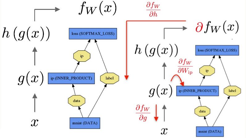
The data xx is passed through an inner product layer for g(x) then through a softmax for h(g(x)) and softmax loss to give fW(x)——表明全连接层到softmax是有参数的，SoftmaxWithLoss相当于一个全连接层连接着一个损失层。

caffe通过solver调用forward计算net的输出以及损失，然后调用backward来计算模型的梯度，然后更新每层的参数使得损失最小。这种net，blob，solver分离的方式使得caffe更模块化，易于开发。

Loss weights

caffe中有loss后缀的层隐含的有一个loss_weight=1参数，其他层隐含的有一个loss_weight=0参数.
如果一个网络有一个SoftmaxWithLoss层进行分类，有一个EuclideanLoss进行重构，那么此时需要使用loss_weight来指定它们的相对重要性。此时我们可以将loss_weight设置为介于0到1之间的数，表示这两个损失函数的重要性。网络整个的损失函数将是所有损失函数的加权和：

loss := 0
for layer in layers:
  for top, loss_weight in layer.tops, layer.loss_weights:
    loss += loss_weight * sum(top)

Solver

caffe的Solver有如下几种：简单介绍SGD

1.Stochastic Gradient Descent (type: “SGD”)

更新公式如下：
Vt+1=μVt−α∇L(Wt) （Vt是前一次梯度更新的量：是负值，V1=−α∇L(W0)）
Wt+1=Wt+Vt+1

设置α，μ的经验是：初始化α≈0.01=10−2，当损失值到达平缓期时将α缩小一个常数倍（比如10），重复多次。μ=0.9或者一个相似的值并且保持不变。动量momentum使得权重的更新更平滑，使得SGD迭代更稳定收敛更快。

在solver.prototxt中设置如下：

base_lr: 0.01     # begin training at a learning rate of 0.01 = 1e-2

lr_policy: "step" # learning rate policy: drop the learning rate in "steps"
                  # by a factor of gamma every stepsize iterations

gamma: 0.1        # drop the learning rate by a factor of 10
                  # (i.e., multiply it by a factor of gamma = 0.1)

stepsize: 100000  # drop the learning rate every 100K iterations

max_iter: 350000  # train for 350K iterations total

momentum: 0.9

注意：动量的存在使得多次迭代后，你的权值更新是没有动量的1/1-μ倍，因此当你的μ=0.9时，多次迭代后，权值更新是传统的是10，如果你将μ=0.99，那么是传统的100倍，因此，你需要相应的将α减小10倍（反之亦然）。

当然上面仅仅是一个指导方针，具体情况具体对待。如果你的训练过程是发散的（损失值或者输出是很大或者Inf或者是NaN），则减小base_lr(比如base_lr: 0.001)，重复试验，直到找到一个合适的base_lr。

2.AdaDelta (type: “AdaDelta”)
3.Adaptive Gradient (type: “AdaGrad”),
4.Adam (type:”Adam”),
5.Nesterov’s Accelerated Gradient (type: “Nesterov”)
6. RMSprop (type: “RMSProp”)

Snapshotting and Resuming

Solver的两个方法Solver::Snapshot()和Solver::SnapshotSolverState()使得我们再训练过程中可以对模型的权重以及solver的状态进行快照，并保存下来。

# The snapshot interval in iterations.
snapshot: 5000
# File path prefix for snapshotting model weights and solver state.
# Note: this is relative to the invocation of the `caffe` utility, not the
# solver definition file.
snapshot_prefix: "/path/to/model"
# Snapshot the diff along with the weights. This can help debugging training
# but takes more storage.
snapshot_diff: false
# A final snapshot is saved at the end of training unless
# this flag is set to false. The default is true.
snapshot_after_train: true

Vision Layers视觉层

Convolution（Convolution）

num_output (c_o)（Required）: the number of filters
kernel_size （Required）: specifies height and width of each filter
weight_filler [default type: ‘constant’ value: 0]：卷积核权重
bias_term [default true]: 指定是否对卷积核添加偏差项
pad (or pad_h and pad_w) [default 0]
stride (or stride_h and stride_w) [default 1]
group (g) [default 1]: If g > 1, 输入和输出channel被分为g组，然后第i个输出组channel与第i个输入组channel相连。

Input：n * c_i * h_i * w_i Output： h_o = h_i + 2 * pad_h - kernel_h) /
stride_h + 1（w_o= w_i + 2 * pad_w - kernel_w) / stride_w + 1）

layer {
  name: "conv1"
  type: "Convolution"
  bottom: "data"
  top: "conv1"
  # learning rate and decay multipliers for the filters
  param { lr_mult: 1 decay_mult: 1 }
  # learning rate and decay multipliers for the biases
  param { lr_mult: 2 decay_mult: 0 }
  convolution_param {
    num_output: 96     # learn 96 filters
    kernel_size: 11    # each filter is 11x11
    stride: 4          # step 4 pixels between each filter application
    weight_filler {
      type: "gaussian" # initialize the filters from a Gaussian
      std: 0.01        # distribution with stdev 0.01 (default mean: 0)
    }
    bias_filler {
      type: "constant" # initialize the biases to zero (0)
      value: 0
    }
  }
}

Pooling（Pooling）

kernel_size （Required）：(h,w)
pool [default MAX]: the pooling method. Currently MAX, AVE, or
STOCHASTIC
pad (or pad_h and pad_w) [default 0]
stride (or stride_h and stride_w) [default 1]

Input：n * c * h_i * w_i Output：h_o = h_i + 2 * pad_h - kernel_h) /
stride_h + 1（w_o= w_i + 2 * pad_w - kernel_w) / stride_w + 1）

layer {
  name: "pool1"
  type: "Pooling"
  bottom: "conv1"
  top: "pool1"
  pooling_param {
    pool: MAX
    kernel_size: 3 # pool over a 3x3 region
    stride: 2      # step two pixels (in the bottom blob) between pooling regions
  }
}

Local Response Normalization (LRN)

局部响应归一化（作用类似侧抑制:lateral inhibition），在输入的局部区域进行归一化操作，公式如下（其中n表示局部区域的大小）：

这里写图片描述

local_size [default 5]：当norm_region=ACROSS_CHANNELS时，该值表示求和的channel的数目。当norm_region=WITHIN_CHANNEL时，该值表示求和的正方形的边长。
alpha [default 1]
beta [default 5]
norm_region [default ACROSS_CHANNELS]：ACROSS_CHANNELS是在相邻的local_size 个channel之间对每个channel的一个元素进行归一化（ local_size x 1 x 1）。WITHIN_CHANNEL 是在一个channel的相邻区域local_size x local_size进行归一化，对这local_size x local_size个元素进行归一化（ 1 x local_size x local_size）。归一化就是局部区域中的每一个元素都除以上面那个求和公式。

Loss Layers损失层

Softmax（SoftmaxWithLoss）

理论上它像是一个softmax 后面跟了一个多项逻辑损失层，但是它提供了更数值稳定的梯度。

Sum-of-Squares / Euclidean（EuclideanLoss）

计算输入和输出的欧氏距离作为损失函数。

Hinge / Margin（HingeLoss）

计算的是一个one-vs-all的平方损失。

norm [default L1]: the norm used. Currently L1, L2

# L1 Norm
layer {
  name: "loss"
  type: "HingeLoss"
  bottom: "pred"
  bottom: "label"
}

# L2 Norm
layer {
  name: "loss"
  type: "HingeLoss"
  bottom: "pred"
  bottom: "label"
  top: "loss"
  hinge_loss_param {
    norm: L2
  }
}

还有一些损失层：SigmoidCrossEntropyLoss，InfogainLoss，Accuracy and Top-k。

Activation / Neuron Layers激活层

ReLU / Rectified-Linear and Leaky-ReLU（ReLU）

negative_slope [default 0]: 将小于0的部分乘以negative_slope 而不是设置为0（标准的ReLU：max(x, 0)）.

layer {
  name: "relu1"
  type: "ReLU"
  bottom: "conv1"
  top: "conv1"
}

Sigmoid（Sigmoid）

对输入x计算 sigmoid(x)

layer {
  name: "encode1neuron"
  bottom: "encode1"
  top: "encode1neuron"
  type: "Sigmoid"
}

TanH / Hyperbolic Tangent（TanH）

对于输入计算 tanh(x)

layer {
  name: "layer"
  bottom: "in"
  top: "out"
  type: "TanH"
}

Absolute Value（AbsVal）

对输入计算abs(x)

layer {
  name: "layer"
  bottom: "in"
  top: "out"
  type: "AbsVal"
}

Power（Power）

对输入计算(shift + scale * x) ^ power
- power [default 1]，scale [default 1]，shift [default 0]

layer {
  name: "layer"
  bottom: "in"
  top: "out"
  type: "Power"
  power_param {
    power: 1
    scale: 1
    shift: 0
  }
}

BNLL（BNLL）

对输入计算 log(1 + exp(x))

layer {
  name: "layer"
  bottom: "in"
  top: "out"
  type: BNLL
}

Data Layers

Database（Data）

source（Required）：包含数据库的文件夹地址（可以是caffe安装位置的相对路径）
batch_size（Required）：一次输入的样本数量
rand_skip: 跳过输入的前rand_skip行，在异步sgd时有用。
backend [default LEVELDB]: LEVELDB/LMDB

In-Memory（MemoryData）

batch_size, channels, height, width（Required）: specify the size of input chunks to read from memory（在python中调用 Net.set_input_arrays来直接从内存读取数据，而不需要从磁盘将数据copy到内存中）。

HDF5 Input（HDF5Data）

HDF5输入层从硬盘中读取HDF5格式的数据。

source（Required）: the name of the file to read from
batch_size（Required）

HDF5 Output（HDF5Output）

HDF5 输出层将其输入blobs以HDF5的格式写入到硬盘中。

file_name（Required）: name of file to write to

Images（ImageData）

source（Required）: 一个文本文本文件，每一行包含图片的名字以及标签
batch_size（Required）
rand_skip
shuffle [default false]
new_height, new_width: if provided, resize all images to this size
还有WindowData以及DummyData 这些数据层。

Common Layers

Inner Product（InnerProduct）

Inner Product（fully connected）全连接层将输入看做简单的向量，然后将其输出为一个单向量（blob的h和w都是1）。

num_output (c_o)（Required）
weight_filler [default type: ‘constant’ value: 0]（Strongly recommended）
bias_filler [default type: ‘constant’ value: 0]
bias_term [default true]: 是否有偏差项

layer {
  name: "fc8"
  type: "InnerProduct"
  # learning rate and decay multipliers for the weights
  param { lr_mult: 1 decay_mult: 1 }
  # learning rate and decay multipliers for the biases
  param { lr_mult: 2 decay_mult: 0 }
  inner_product_param {
    num_output: 1000
    weight_filler {
      type: "gaussian"
      std: 0.01
    }
    bias_filler {
      type: "constant"
      value: 0
    }
  }
  bottom: "fc7"
  top: "fc8"
}

Splitting

分离层是一个功能层，将一个输入blob分裂为多个blob输出，通常需要将一个blob作为多个层的输入是需要使用该层。

Flattening

平滑层是一个功能层，将一个形如n*c*h*w的输入处理为一个单向量：n*(c*h*w).

Reshape（Reshape）

Reshape形变层用来改变输入的维度，但是不改变数据元素的个数。这个过程中只改变了维度，没有数据的复制。

0：表示复制输入blob该位置的维度大小，比如bottom的blob是2*，然后让dim: 0 那么输出也是2*n.
-1：根据其它已经确定好的维度，推测该位置的维度大小。

 layer {
    name: "reshape"
    type: "Reshape"
    bottom: "input"
    top: "output"
    reshape_param {
      shape {
        dim: 0  # copy the dimension from below
        dim: 2
        dim: 3
        dim: -1 # infer it from the other dimensions
      }
    }
  }

一个特殊的设置：将第一个维度保持不变，其它维度自己调整。这个和Flatten的效果一样，转化为一个单向量（n，c*h*w）

shape { dim: 0 dim: -1 }

Concatenation（Concat）

Concatenation连接层是一个功能层，将多个输入blob连接成一个单独的输出blob.

Input：n_i * c_i * h * w for each input blob i from 1 to K.
Output：多个blob的h和w必须一样
- if axis = 0: (n_1 + n_2 + … + n_K) * c_1 * h * w, and all input c_i should be the same（c相同，就是累积对n求和）.
- if axis = 1: n_1 * (c_1 + c_2 + … + c_K) * h * w, and all input n_i should be the same（n相同，就是累积对c求和）.

layer {
  name: "concat"
  bottom: "in1"
  bottom: "in2"
  top: "out"
  type: "Concat"
  concat_param {
    axis: 1
  }
}

Slicing（Slice）

Slice 切片层是一个功能层，对一个输入blob根据给定的维度(只支持n和c)进行切片，得到多个输出blob.

axis 表示目标轴，slice_point 表示要进行切片的维度的下标（index的个数必须等于top blobs的数目-1）

layer {
  name: "slicer_label"
  type: "Slice"
  bottom: "label"
  ## Example of label with a shape N x 3 x 1 x 1
  top: "label1"
  top: "label2"
  top: "label3"
  slice_param {
    axis: 1
    slice_point: 1
    slice_point: 2
  }
}

mmい

关注

0
点赞
踩
1

收藏

觉得还不错? 一键收藏
0
评论
caffe基础

Blob 大多数caffe blob是4D的，格式为：N*K*H*W N：batch的大小，表示每次训练N个数据样本就进行一次梯度下降(ImageNet 数据集的训练batch=256). K ：数据特征的维度，比如输入RGB图像，那么K=3. 下标为(n, k, h, w)的元素的物理地址为((n * K + k) * H + h) * W + w 也有2D的，格
复制链接

扫一扫