灰度共生矩阵（GLCM）并计算能量、熵、惯性矩、相关性（matlab）（待总结）

最新推荐文章于 2024-04-19 14:13:59 发布

zoukangdlut

最新推荐文章于 2024-04-19 14:13:59 发布

阅读量1w

点赞数 1

关于灰度共生矩阵的介绍可参考

http://blog.csdn.net/chuminnan2010/article/details/22035751

http://blog.csdn.net/xuezhisd/article/details/8908824

http://blog.csdn.net/xuexiang0704/article/details/8713204

http://cn.mathworks.com/help/images/ref/imlincomb.html?refresh=true

理论介绍

http://blog.csdn.net/lskyne/article/details/8659225
http://blog.csdn.net/light_lj/article/details/26098815
http://blog.csdn.net/kezunhai/article/details/42001477

共生矩阵的物理意义
http://blog.csdn.net/light_lj/article/details/26098815

下面给出不同的NumLevels的例子

gray = [1 1 5 6 8  
        2 3 5 7 1  
        4 5 7 1 2  
        8 5 1 2 5];
GLCM = graycomatrix(gray,'GrayLimits',[])

GLCM =

     1     2     0     0     1     0     0     0
     0     0     1     0     1     0     0     0
     0     0     0     0     1     0     0     0
     0     0     0     0     1     0     0     0
     1     0     0     0     0     1     2     0
     0     0     0     0     0     0     0     1
     2     0     0     0     0     0     0     0
     0     0     0     0     1     0     0     0


GLCM = graycomatrix(gray, 'GrayLimits',[],'offset', [0 1])

GLCM =

     1     2     0     0     1     0     0     0
     0     0     1     0     1     0     0     0
     0     0     0     0     1     0     0     0
     0     0     0     0     1     0     0     0
     1     0     0     0     0     1     2     0
     0     0     0     0     0     0     0     1
     2     0     0     0     0     0     0     0
     0     0     0     0     1     0     0     0

GLCM = graycomatrix(gray, 'GrayLimits',[],'offset', [0 1],'NumLevels',8)

GLCM =

     1     2     0     0     1     0     0     0
     0     0     1     0     1     0     0     0
     0     0     0     0     1     0     0     0
     0     0     0     0     1     0     0     0
     1     0     0     0     0     1     2     0
     0     0     0     0     0     0     0     1
     2     0     0     0     0     0     0     0
     0     0     0     0     1     0     0     0
 
 1
2
3
4
5
6
7
8
9
10
11
12
13
14
15
16
17
18
19
20
21
22
23
24
25
26
27
28
29
30
31
32
33
34
35
36
37
38
39
40
41
42
43
 
 1
2
3
4
5
6
7
8
9
10
11
12
13
14
15
16
17
18
19
20
21
22
23
24
25
26
27
28
29
30
31
32
33
34
35
36
37
38
39
40
41
42
43

这里写图片描述

上图显示了如何求解灰度共生矩阵，以（1，1）点为例，GLCM（1，1）值为1说明只有一对灰度为1的像素水平相邻。GLCM（1，2）值为2，是因为有两对灰度为1和2的像素水平相邻。（1,5）出现一次，所以在（1.5）位置上标记1，没出现（1,6)所以为0；

上面所有的参数都是默认设置，NumLevels=8，下面考虑NumLevels=3 的情况

gray = [1 1 5 6 8  
        2 3 5 7 1  
        4 5 7 1 2  
        8 5 1 2 5];

GL(2) = max(max(gray));
GL(1) = min(min(gray));
if GL(2) == GL(1)
  SI = ones(size(gray));
else 
    slope = NumLevels/(GL(2) - GL(1));
    intercept = 1 - (slope*(GL(1)));
    SI = floor(imlincomb(slope,gray,intercept,'double'));
end
%%%%%%%%%%%%%%%%%%%%%%%%%%%%%%%%%%%%%%%%%%%%%%%%%%%%%%%%%
SI =

     1     1     2     3     4
     1     1     2     3     1
     2     2     3     1     1
     4     2     1     1     2
%%%%%%%%%%%%%%%%%%%%%%%%%%%%%%%%%%%%%%%%%%%%%%%%%%%%%%%%%%


SI(SI > NumLevels) = NumLevels;
SI(SI < 1) = 1;

SI =

     1     1     2     3     3
     1     1     2     3     1
     2     2     3     1     1
     3     2     1     1     2
 
 1
2
3
4
5
6
7
8
9
10
11
12
13
14
15
16
17
18
19
20
21
22
23
24
25
26
27
28
29
30
31
32
33
 
 1
2
3
4
5
6
7
8
9
10
11
12
13
14
15
16
17
18
19
20
21
22
23
24
25
26
27
28
29
30
31
32
33

上面给出了如何将初始矩阵gray变成3阶的灰度级，SI就是gray的3阶灰度级矩阵。

这里写图片描述

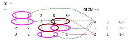
上图显示了如何求解3级灰度共生矩阵，以（1，1）点为例，GLCM（1，1）值为4说明只有4对灰度为1的像素水平相邻。GLCM（3，1）值为2，是因为有两对灰度为3和1的像素水平相邻。（2,1）出现一次，所以在（2.1）位置上标记1，没出现（1,3)所以为0；

gray = [1 1 5 6 8  
        2 3 5 7 1  
        4 5 7 1 2  
        8 5 1 2 5];
[GLCM,SI] = graycomatrix(gray,'NumLevels',3,'G',[])

GLCM =

     4     3     0
     1     1     3
     2     1     1


SI =

     1     1     2     3     3
     1     1     2     3     1
     2     2     3     1     1
     3     2     1     1     2
 
 1
2
3
4
5
6
7
8
9
10
11
12
13
14
15
16
17
18
19
 
 1
2
3
4
5
6
7
8
9
10
11
12
13
14
15
16
17
18
19

用3阶灰度级去计算四个共生矩阵P,取距离为1，角度分别为0,45,90,135

gray = [1 1 5 6 8
    2 3 5 7 1
    4 5 7 1 2
    8 5 1 2 5];
offsets = [0 1;-1 1;-1 0;-1 -1];
m = 3; % 3阶灰度级
[GLCMS,SI] = graycomatrix(gray,'GrayLimits',[],'Of',offsets,'NumLevels',m);
P = GLCMS;
[kk,ll,mm] = size(P);
% 对共生矩阵归一化
%---------------------------------------------------------
for n = 1:mm
    P(:,:,n) = P(:,:,n)/sum(sum(P(:,:,n)));
end

%-----------------------------------------------------------
%对共生矩阵计算能量、熵、惯性矩、相关4个纹理参数
%-----------------------------------------------------------
H = zeros(1,mm);
I = H;
Ux = H;      Uy = H;
deltaX= H;  deltaY = H;
C =H;
for n = 1:mm
    E(n) = sum(sum(P(:,:,n).^2)); %能量
    for i = 1:kk
        for j = 1:ll
            if P(i,j,n)~=0
                H(n) = -P(i,j,n)*log(P(i,j,n))+H(n); %熵
            end
            I(n) = (i-j)^2*P(i,j,n)+I(n);  %惯性矩

            Ux(n) = i*P(i,j,n)+Ux(n); %相关性中μx
            Uy(n) = j*P(i,j,n)+Uy(n); %相关性中μy
        end
    end
end
for n = 1:mm
    for i = 1:kk
        for j = 1:ll
            deltaX(n) = (i-Ux(n))^2*P(i,j,n)+deltaX(n); %相关性中σx
            deltaY(n) = (j-Uy(n))^2*P(i,j,n)+deltaY(n); %相关性中σy
            C(n) = i*j*P(i,j,n)+C(n);
        end
    end
    C(n) = (C(n)-Ux(n)*Uy(n))/deltaX(n)/deltaY(n); %相关性
end

%--------------------------------------------------------------------------
%求能量、熵、惯性矩、相关的均值和标准差作为最终8维纹理特征
%--------------------------------------------------------------------------
a1 = mean(E)
b1 = sqrt(cov(E))

a2 = mean(H)
b2 = sqrt(cov(H))

a3 = mean(I)
b3 = sqrt(cov(I))

a4 = mean(C)
b4 = sqrt(cov(C))

sprintf('0,45,90,135方向上的能量依次为： %f, %f, %f, %f',E(1),E(2),E(3),E(4))  % 输出数据;
sprintf('0,45,90,135方向上的熵依次为： %f, %f, %f, %f',H(1),H(2),H(3),H(4))  % 输出数据;
sprintf('0,45,90,135方向上的惯性矩依次为： %f, %f, %f, %f',I(1),I(2),I(3),I(4))  % 输出数据;
sprintf('0,45,90,135方向上的相关性依次为： %f, %f, %f, %f',C(1),C(2),C(3),C(4))  % 输出数据;


 
 1
2
3
4
5
6
7
8
9
10
11
12
13
14
15
16
17
18
19
20
21
22
23
24
25
26
27
28
29
30
31
32
33
34
35
36
37
38
39
40
41
42
43
44
45
46
47
48
49
50
51
52
53
54
55
56
57
58
59
60
61
62
63
64
65
66
67
68
69
 
 1
2
3
4
5
6
7
8
9
10
11
12
13
14
15
16
17
18
19
20
21
22
23
24
25
26
27
28
29
30
31
32
33
34
35
36
37
38
39
40
41
42
43
44
45
46
47
48
49
50
51
52
53
54
55
56
57
58
59
60
61
62
63
64
65
66
67
68
69

下面给出的是默认的设置下求四个方向的灰度共生矩阵，NumLevels=8.

gray = [1 1 5 6 8  
        2 3 5 7 1  
        4 5 7 1 2  
        8 5 1 2 5];
offsets = [0 1;-1 1;-1 0;-1 -1];
[GLCMS,SI] = graycomatrix(gray,'GrayLimits',[],'Of',offsets)

GLCMS(:,:,1) =

     1     2     0     0     1     0     0     0
     0     0     1     0     1     0     0     0
     0     0     0     0     1     0     0     0
     0     0     0     0     1     0     0     0
     1     0     0     0     0     1     2     0
     0     0     0     0     0     0     0     1
     2     0     0     0     0     0     0     0
     0     0     0     0     1     0     0     0


GLCMS(:,:,2) =

     2     0     0     0     0     0     0     0
     1     1     0     0     0     0     0     0
     0     0     0     0     1     0     0     0
     0     0     1     0     0     0     0     0
     0     0     0     0     1     1     1     0
     0     0     0     0     0     0     0     0
     0     0     0     0     0     0     1     1
     0     0     0     0     1     0     0     0


GLCMS(:,:,3) =

     0     0     0     0     0     0     2     1
     3     0     0     0     0     0     0     0
     1     0     0     0     0     0     0     0
     0     1     0     0     0     0     0     0
     0     1     1     0     2     0     0     0
     0     0     0     0     0     0     0     0
     0     0     0     0     1     1     0     0
     0     0     0     1     0     0     0     0


GLCMS(:,:,4) =

     0     0     0     0     2     1     0     0
     0     0     0     0     0     0     2     0
     1     0     0     0     0     0     0     0
     0     0     0     0     0     0     0     0
     2     1     0     1     0     0     0     0
     0     0     0     0     0     0     0     0
     0     0     1     0     1     0     0     0
     0     0     0     0     0     0     0     0


SI =

     1     1     5     6     8
     2     3     5     7     1
     4     5     7     1     2
     8     5     1     2     5

 
 1
2
3
4
5
6
7
8
9
10
11
12
13
14
15
16
17
18
19
20
21
22
23
24
25
26
27
28
29
30
31
32
33
34
35
36
37
38
39
40
41
42
43
44
45
46
47
48
49
50
51
52
53
54
55
56
57
58
59
60
61
62
 
 1
2
3
4
5
6
7
8
9
10
11
12
13
14
15
16
17
18
19
20
21
22
23
24
25
26
27
28
29
30
31
32
33
34
35
36
37
38
39
40
41
42
43
44
45
46
47
48
49
50
51
52
53
54
55
56
57
58
59
60
61
62

下面给出更多的关于灰度共生矩阵的特征

I = imread('circuit.tif');
GLCM2 = graycomatrix(I,'GrayLimits',[],'Offset',[0 1;-1 1;-1 0;-1 -1]);
stats = GLCM_Features1(GLCM2,0)
 
 1
2
3
 
 1
2
3

I = imread('circuit.tif');
AllGLCMFeatureb= caluateglcmfeature(I);
 
 1
2
 
 1
2

function [newglcm] = caluateglcmfeature(I);
GLCM2 = graycomatrix(I,'GrayLimits',[],'Offset',[0 1;-1 1;-1 0;-1 -1]);
stats = GLCM_Features1(GLCM2,0)
newstats = struct2cell(stats);
[statsx,statsy] = size(newstats);
newglcm = [];
for i = 1:statsx
    element = [];
    newelement = [];
    glcm = [];
    element = newstats(i,1);
    newelement = element{1,1};
    average = mean(newelement);
    variance = sqrt(cov(newelement));
    glcm = [newelement average variance];
    newglcm = [newglcm glcm];
end
end
 
 1
2
3
4
5
6
7
8
9
10
11
12
13
14
15
16
17
18
 
 1
2
3
4
5
6
7
8
9
10
11
12
13
14
15
16
17
18

% http://www.mathworks.com/matlabcentral/fileexchange/22187-glcm-texture-features
% This code from the upper website but we have changed some.
function [out] = GLCM_Features1(glcmin,pairs)
% GLCM_Features1 helps to calculate the features from the different GLCMs
% that are input to the function. The GLCMs are stored in a i x j x n
% matrix, where n is the number of GLCMs calculated usually due to the
% different orientation and displacements used in the algorithm. Usually
% the values i and j are equal to 'NumLevels' parameter of the GLCM
% computing function graycomatrix(). Note that matlab quantization values
% belong to the set {1,..., NumLevels} and not from {0,...,(NumLevels-1)}
% as provided in some references
% http://www.mathworks.com/access/helpdesk/help/toolbox/images/graycomatrix
% .html
% 
% Although there is a function graycoprops() in Matlab Image Processing
% Toolbox that computes four parameters Contrast, Correlation, Energy,
% and Homogeneity. The paper by Haralick suggests a few more parameters
% that are also computed here. The code is not fully vectorized and hence
% is not an efficient implementation but it is easy to add new features
% based on the GLCM using this code. Takes care of 3 dimensional glcms
% (multiple glcms in a single 3D array)
% 
% If you find that the values obtained are different from what you expect 
% or if you think there is a different formula that needs to be used 
% from the ones used in this code please let me know. 
% A few questions which I have are listed in the link 
% http://www.mathworks.com/matlabcentral/newsreader/view_thread/239608
%
% I plan to submit a vectorized version of the code later and provide 
% updates based on replies to the above link and this initial code. 
%
% Features computed 
% Autocorrelation: [2]                      (out.autoc)
% Contrast: matlab/[1,2]                    (out.contr)
% Correlation: matlab                       (out.corrm)
% Correlation: [1,2]                        (out.corrp)
% Cluster Prominence: [2]                   (out.cprom)
% Cluster Shade: [2]                        (out.cshad)
% Dissimilarity: [2]                        (out.dissi)
% Energy: matlab / [1,2]                    (out.energ)
% Entropy: [2]                              (out.entro)
% Homogeneity: matlab                       (out.homom)
% Homogeneity: [2]                          (out.homop)
% Maximum probability: [2]                  (out.maxpr)
% Sum of sqaures: Variance [1]              (out.sosvh)
% Sum average [1]                           (out.savgh)
% Sum variance [1]                          (out.svarh)
% Sum entropy [1]                           (out.senth)
% Difference variance [1]                   (out.dvarh)
% Difference entropy [1]                    (out.denth)
% Information measure of correlation1 [1]   (out.inf1h)
% Informaiton measure of correlation2 [1]   (out.inf2h)
% Inverse difference (INV) is homom [3]     (out.homom)
% Inverse difference normalized (INN) [3]   (out.indnc) 
% Inverse difference moment normalized [3]  (out.idmnc)
%
% The maximal correlation coefficient was not calculated due to
% computational instability 
% http://murphylab.web.cmu.edu/publications/boland/boland_node26.html
%
% Formulae from MATLAB site (some look different from
% the paper by Haralick but are equivalent and give same results)
% Example formulae: 
% Contrast = sum_i(sum_j(  (i-j)^2 * p(i,j) ) ) (same in matlab/paper)
% Correlation = sum_i( sum_j( (i - u_i)(j - u_j)p(i,j)/(s_i.s_j) ) ) (m)
% Correlation = sum_i( sum_j( ((ij)p(i,j) - u_x.u_y) / (s_x.s_y) ) ) (p[2])
% Energy = sum_i( sum_j( p(i,j)^2 ) )           (same in matlab/paper)
% Homogeneity = sum_i( sum_j( p(i,j) / (1 + |i-j|) ) ) (as in matlab)
% Homogeneity = sum_i( sum_j( p(i,j) / (1 + (i-j)^2) ) ) (as in paper)
% 
% Where:
% u_i = u_x = sum_i( sum_j( i.p(i,j) ) ) (in paper [2])
% u_j = u_y = sum_i( sum_j( j.p(i,j) ) ) (in paper [2])
% s_i = s_x = sum_i( sum_j( (i - u_x)^2.p(i,j) ) ) (in paper [2])
% s_j = s_y = sum_i( sum_j( (j - u_y)^2.p(i,j) ) ) (in paper [2])
%
% 
% Normalize the glcm:
% Compute the sum of all the values in each glcm in the array and divide 
% each element by it sum
%
% Haralick uses 'Symmetric' = true in computing the glcm
% There is no Symmetric flag in the Matlab version I use hence
% I add the diagonally opposite pairs to obtain the Haralick glcm
% Here it is assumed that the diagonally opposite orientations are paired
% one after the other in the matrix
% If the above assumption is true with respect to the input glcm then
% setting the flag 'pairs' to 1 will compute the final glcms that would result 
% by setting 'Symmetric' to true. If your glcm is computed using the
% Matlab version with 'Symmetric' flag you can set the flag 'pairs' to 0
%
% References:
% 1. R. M. Haralick, K. Shanmugam, and I. Dinstein, Textural Features of
% Image Classification, IEEE Transactions on Systems, Man and Cybernetics,
% vol. SMC-3, no. 6, Nov. 1973
% 2. L. Soh and C. Tsatsoulis, Texture Analysis of SAR Sea Ice Imagery
% Using Gray Level Co-Occurrence Matrices, IEEE Transactions on Geoscience
% and Remote Sensing, vol. 37, no. 2, March 1999.
% 3. D A. Clausi, An analysis of co-occurrence texture statistics as a
% function of grey level quantization, Can. J. Remote Sensing, vol. 28, no.
% 1, pp. 45-62, 2002
% 4. http://murphylab.web.cmu.edu/publications/boland/boland_node26.html
%
%
% Example:
%
% Usage is similar to graycoprops() but needs extra parameter 'pairs' apart
% from the GLCM as input
% I = imread('circuit.tif');
% GLCM2 = graycomatrix(I,'GrayLimits',[],'Offset',[0 1;-1 1;-1 0;-1 -1]);
% stats = GLCM_Features1(GLCM2,0)
% The output is a structure containing all the parameters for the different
% GLCMs
%
% [Avinash Uppuluri: avinash_uv@yahoo.com: Last modified: 11/20/08]

% If 'pairs' not entered: set pairs to 0 
if ((nargin > 2) || (nargin == 0))
   error('Too many or too few input arguments. Enter GLCM and pairs.');
elseif ( (nargin == 2) ) 
    if ((size(glcmin,1) <= 1) || (size(glcmin,2) <= 1))
       error('The GLCM should be a 2-D or 3-D matrix.');
    elseif ( size(glcmin,1) ~= size(glcmin,2) )
        error('Each GLCM should be square with NumLevels rows and NumLevels cols');
    end    
elseif (nargin == 1) % only GLCM is entered
    pairs = 0; % default is numbers and input 1 for percentage
    if ((size(glcmin,1) <= 1) || (size(glcmin,2) <= 1))
       error('The GLCM should be a 2-D or 3-D matrix.');
    elseif ( size(glcmin,1) ~= size(glcmin,2) )
       error('Each GLCM should be square with NumLevels rows and NumLevels cols');
    end    
end


format long e
if (pairs == 1)
    newn = 1;
    for nglcm = 1:2:size(glcmin,3)
        glcm(:,:,newn)  = glcmin(:,:,nglcm) + glcmin(:,:,nglcm+1);
        newn = newn + 1;
    end
elseif (pairs == 0)
    glcm = glcmin;
end

size_glcm_1 = size(glcm,1);
size_glcm_2 = size(glcm,2);
size_glcm_3 = size(glcm,3);

% checked 
out.autoc = zeros(1,size_glcm_3); % Autocorrelation: [2] 
out.contr = zeros(1,size_glcm_3); % Contrast: matlab/[1,2]
out.corrm = zeros(1,size_glcm_3); % Correlation: matlab
out.corrp = zeros(1,size_glcm_3); % Correlation: [1,2]
out.cprom = zeros(1,size_glcm_3); % Cluster Prominence: [2]
out.cshad = zeros(1,size_glcm_3); % Cluster Shade: [2]
out.dissi = zeros(1,size_glcm_3); % Dissimilarity: [2]
out.energ = zeros(1,size_glcm_3); % Energy: matlab / [1,2]
out.entro = zeros(1,size_glcm_3); % Entropy: [2]
out.homom = zeros(1,size_glcm_3); % Homogeneity: matlab
out.homop = zeros(1,size_glcm_3); % Homogeneity: [2]
out.maxpr = zeros(1,size_glcm_3); % Maximum probability: [2]

out.sosvh = zeros(1,size_glcm_3); % Sum of sqaures: Variance [1]
out.savgh = zeros(1,size_glcm_3); % Sum average [1]
out.svarh = zeros(1,size_glcm_3); % Sum variance [1]
out.senth = zeros(1,size_glcm_3); % Sum entropy [1]
out.dvarh = zeros(1,size_glcm_3); % Difference variance [4]
%out.dvarh2 = zeros(1,size_glcm_3); % Difference variance [1]
out.denth = zeros(1,size_glcm_3); % Difference entropy [1]
out.inf1h = zeros(1,size_glcm_3); % Information measure of correlation1 [1]
out.inf2h = zeros(1,size_glcm_3); % Informaiton measure of correlation2 [1]
%out.mxcch = zeros(1,size_glcm_3);% maximal correlation coefficient [1]
%out.invdc = zeros(1,size_glcm_3);% Inverse difference (INV) is homom [3]
out.indnc = zeros(1,size_glcm_3); % Inverse difference normalized (INN) [3]
out.idmnc = zeros(1,size_glcm_3); % Inverse difference moment normalized [3]

% correlation with alternate definition of u and s
%out.corrm2 = zeros(1,size_glcm_3); % Correlation: matlab
%out.corrp2 = zeros(1,size_glcm_3); % Correlation: [1,2]

glcm_sum  = zeros(size_glcm_3,1);
glcm_mean = zeros(size_glcm_3,1);
glcm_var  = zeros(size_glcm_3,1);

% http://www.fp.ucalgary.ca/mhallbey/glcm_mean.htm confuses the range of 
% i and j used in calculating the means and standard deviations.
% As of now I am not sure if the range of i and j should be [1:Ng] or
% [0:Ng-1]. I am working on obtaining the values of mean and std that get
% the values of correlation that are provided by matlab.
u_x = zeros(size_glcm_3,1);
u_y = zeros(size_glcm_3,1);
s_x = zeros(size_glcm_3,1);
s_y = zeros(size_glcm_3,1);

% % alternate values of u and s
% u_x2 = zeros(size_glcm_3,1);
% u_y2 = zeros(size_glcm_3,1);
% s_x2 = zeros(size_glcm_3,1);
% s_y2 = zeros(size_glcm_3,1);

% checked p_x p_y p_xplusy p_xminusy
p_x = zeros(size_glcm_1,size_glcm_3); % Ng x #glcms[1]  
p_y = zeros(size_glcm_2,size_glcm_3); % Ng x #glcms[1]
p_xplusy = zeros((size_glcm_1*2 - 1),size_glcm_3); %[1]
p_xminusy = zeros((size_glcm_1),size_glcm_3); %[1]
% checked hxy hxy1 hxy2 hx hy
hxy  = zeros(size_glcm_3,1);
hxy1 = zeros(size_glcm_3,1);
hx   = zeros(size_glcm_3,1);
hy   = zeros(size_glcm_3,1);
hxy2 = zeros(size_glcm_3,1);

%Q    = zeros(size(glcm));

for k = 1:size_glcm_3 % number glcms

    glcm_sum(k) = sum(sum(glcm(:,:,k)));
    glcm(:,:,k) = glcm(:,:,k)./glcm_sum(k); % Normalize each glcm
    glcm_mean(k) = mean2(glcm(:,:,k)); % compute mean after norm
    glcm_var(k)  = (std2(glcm(:,:,k)))^2;

    for i = 1:size_glcm_1

        for j = 1:size_glcm_2

            out.contr(k) = out.contr(k) + (abs(i - j))^2.*glcm(i,j,k);
            out.dissi(k) = out.dissi(k) + (abs(i - j)*glcm(i,j,k));
            out.energ(k) = out.energ(k) + (glcm(i,j,k).^2);
            out.entro(k) = out.entro(k) - (glcm(i,j,k)*log(glcm(i,j,k) + eps));

            out.homom(k) = out.homom(k) + (glcm(i,j,k)/( 1 + abs(i-j) ));
            out.homop(k) = out.homop(k) + (glcm(i,j,k)/( 1 + (i - j)^2));
            % [1] explains sum of squares variance with a mean value;
            % the exact definition for mean has not been provided in 
            % the reference: I use the mean of the entire normalized glcm 
            out.sosvh(k) = out.sosvh(k) + glcm(i,j,k)*((i - glcm_mean(k))^2);

            %out.invdc(k) = out.homom(k);
            out.indnc(k) = out.indnc(k) + (glcm(i,j,k)/( 1 + (abs(i-j)/size_glcm_1) ));
            out.idmnc(k) = out.idmnc(k) + (glcm(i,j,k)/( 1 + ((i - j)/size_glcm_1)^2));
            u_x(k)          = u_x(k) + (i)*glcm(i,j,k); % changed 10/26/08
            u_y(k)          = u_y(k) + (j)*glcm(i,j,k); % changed 10/26/08
            % code requires that Nx = Ny 
            % the values of the grey levels range from 1 to (Ng) 
        end

    end
    out.maxpr(k) = max(max(glcm(:,:,k)));
end
% glcms have been normalized:
% The contrast has been computed for each glcm in the 3D matrix
% (tested) gives similar results to the matlab function

for k = 1:size_glcm_3

    for i = 1:size_glcm_1

        for j = 1:size_glcm_2
            p_x(i,k) = p_x(i,k) + glcm(i,j,k); 
            p_y(i,k) = p_y(i,k) + glcm(j,i,k); % taking i for j and j for i
            if (ismember((i + j),[2:2*size_glcm_1])) 
                p_xplusy((i+j)-1,k) = p_xplusy((i+j)-1,k) + glcm(i,j,k);
            end
            if (ismember(abs(i-j),[0:(size_glcm_1-1)])) 
                p_xminusy((abs(i-j))+1,k) = p_xminusy((abs(i-j))+1,k) +...
                    glcm(i,j,k);
            end
        end
    end

%     % consider u_x and u_y and s_x and s_y as means and standard deviations
%     % of p_x and p_y
%     u_x2(k) = mean(p_x(:,k));
%     u_y2(k) = mean(p_y(:,k));
%     s_x2(k) = std(p_x(:,k));
%     s_y2(k) = std(p_y(:,k));

end

% marginal probabilities are now available [1]
% p_xminusy has +1 in index for matlab (no 0 index)
% computing sum average, sum variance and sum entropy:
for k = 1:(size_glcm_3)

    for i = 1:(2*(size_glcm_1)-1)
        out.savgh(k) = out.savgh(k) + (i+1)*p_xplusy(i,k);
        % the summation for savgh is for i from 2 to 2*Ng hence (i+1)
        out.senth(k) = out.senth(k) - (p_xplusy(i,k)*log(p_xplusy(i,k) + eps));
    end

end
% compute sum variance with the help of sum entropy
for k = 1:(size_glcm_3)

    for i = 1:(2*(size_glcm_1)-1)
        out.svarh(k) = out.svarh(k) + (((i+1) - out.senth(k))^2)*p_xplusy(i,k);
        % the summation for savgh is for i from 2 to 2*Ng hence (i+1)
    end

end
% compute difference variance, difference entropy, 
for k = 1:size_glcm_3
% out.dvarh2(k) = var(p_xminusy(:,k));
% but using the formula in 
% http://murphylab.web.cmu.edu/publications/boland/boland_node26.html
% we have for dvarh
    for i = 0:(size_glcm_1-1)
        out.denth(k) = out.denth(k) - (p_xminusy(i+1,k)*log(p_xminusy(i+1,k) + eps));
        out.dvarh(k) = out.dvarh(k) + (i^2)*p_xminusy(i+1,k);
    end
end

% compute information measure of correlation(1,2) [1]
for k = 1:size_glcm_3
    hxy(k) = out.entro(k);
    for i = 1:size_glcm_1

        for j = 1:size_glcm_2
            hxy1(k) = hxy1(k) - (glcm(i,j,k)*log(p_x(i,k)*p_y(j,k) + eps));
            hxy2(k) = hxy2(k) - (p_x(i,k)*p_y(j,k)*log(p_x(i,k)*p_y(j,k) + eps));
%             for Qind = 1:(size_glcm_1)
%                 Q(i,j,k) = Q(i,j,k) +...
%                     ( glcm(i,Qind,k)*glcm(j,Qind,k) / (p_x(i,k)*p_y(Qind,k)) ); 
%             end
        end
        hx(k) = hx(k) - (p_x(i,k)*log(p_x(i,k) + eps));
        hy(k) = hy(k) - (p_y(i,k)*log(p_y(i,k) + eps));
    end
    out.inf1h(k) = ( hxy(k) - hxy1(k) ) / ( max([hx(k),hy(k)]) );
    out.inf2h(k) = ( 1 - exp( -2*( hxy2(k) - hxy(k) ) ) )^0.5;
%     eig_Q(k,:)   = eig(Q(:,:,k));
%     sort_eig(k,:)= sort(eig_Q(k,:),'descend');
%     out.mxcch(k) = sort_eig(k,2)^0.5;
% The maximal correlation coefficient was not calculated due to
% computational instability 
% http://murphylab.web.cmu.edu/publications/boland/boland_node26.html
end

corm = zeros(size_glcm_3,1);
corp = zeros(size_glcm_3,1);
% using http://www.fp.ucalgary.ca/mhallbey/glcm_variance.htm for s_x s_y
for k = 1:size_glcm_3
    for i = 1:size_glcm_1
        for j = 1:size_glcm_2
            s_x(k)  = s_x(k)  + (((i) - u_x(k))^2)*glcm(i,j,k);
            s_y(k)  = s_y(k)  + (((j) - u_y(k))^2)*glcm(i,j,k);
            corp(k) = corp(k) + ((i)*(j)*glcm(i,j,k));
            corm(k) = corm(k) + (((i) - u_x(k))*((j) - u_y(k))*glcm(i,j,k));
            out.cprom(k) = out.cprom(k) + (((i + j - u_x(k) - u_y(k))^4)*...
                glcm(i,j,k));
            out.cshad(k) = out.cshad(k) + (((i + j - u_x(k) - u_y(k))^3)*...
                glcm(i,j,k));
        end
    end
    % using http://www.fp.ucalgary.ca/mhallbey/glcm_variance.htm for s_x
    % s_y : This solves the difference in value of correlation and might be
    % the right value of standard deviations required 
    % According to this website there is a typo in [2] which provides
    % values of variance instead of the standard deviation hence a square
    % root is required as done below:
    s_x(k) = s_x(k) ^ 0.5;
    s_y(k) = s_y(k) ^ 0.5;
    out.autoc(k) = corp(k);
    out.corrp(k) = (corp(k) - u_x(k)*u_y(k))/(s_x(k)*s_y(k));
    out.corrm(k) = corm(k) / (s_x(k)*s_y(k));
%     % alternate values of u and s
%     out.corrp2(k) = (corp(k) - u_x2(k)*u_y2(k))/(s_x2(k)*s_y2(k));
%     out.corrm2(k) = corm(k) / (s_x2(k)*s_y2(k));
end
%--------------------------------------------------------------------------

% Here the formula in the paper out.corrp and the formula in matlab
% out.corrm are equivalent as confirmed by the similar results obtained

% % The papers have a slightly different formular for Contrast
% % I have tested here to find this formula in the papers provides the 
% % same results as the formula provided by the matlab function for 
% % Contrast (Hence this part has been commented)
% out.contrp = zeros(size_glcm_3,1);
% contp = 0;
% Ng = size_glcm_1;
% for k = 1:size_glcm_3
%     for n = 0:(Ng-1)
%         for i = 1:Ng
%             for j = 1:Ng
%                 if (abs(i-j) == n)
%                     contp = contp + glcm(i,j,k);
%                 end
%             end
%         end
%         out.contrp(k) = out.contrp(k) + n^2*contp;
%         contp = 0;
%     end
%     
% end

%       GLCM Features (Soh, 1999; Haralick, 1973; Clausi 2002)
%           f1. Uniformity / Energy / Angular Second Moment (done)
%           f2. Entropy (done)
%           f3. Dissimilarity (done)
%           f4. Contrast / Inertia (done)
%           f5. Inverse difference    
%           f6. correlation
%           f7. Homogeneity / Inverse difference moment
%           f8. Autocorrelation
%           f9. Cluster Shade
%          f10. Cluster Prominence
%          f11. Maximum probability
%          f12. Sum of Squares
%          f13. Sum Average
%          f14. Sum Variance
%          f15. Sum Entropy
%          f16. Difference variance
%          f17. Difference entropy
%          f18. Information measures of correlation (1)
%          f19. Information measures of correlation (2)
%          f20. Maximal correlation coefficient
%          f21. Inverse difference normalized (INN)
%          f22. Inverse difference moment normalized (IDN)

zoukangdlut

关注

1
点赞
踩
26

收藏

觉得还不错? 一键收藏
0
评论
灰度共生矩阵（GLCM）并计算能量、熵、惯性矩、相关性（matlab）（待总结）

关于灰度共生矩阵的介绍可参考http://blog.csdn.net/chuminnan2010/article/details/22035751http://blog.csdn.net/xuezhisd/article/details/8908824http://blog.csdn.net/xuexiang0704/article/details/8713204h
复制链接

扫一扫