


【CFD理论】对流项-02
知识回顾
a
E
=
D
−
F
2
a_E=D-\frac{F}{2}
aE=D−2F
a
W
=
D
+
F
2
a_W=D+\frac{F}{2}
aW=D+2F
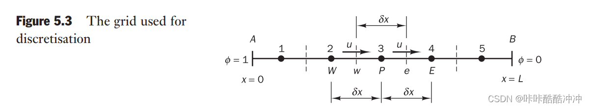
边界问题
Dirichlet
Newmann
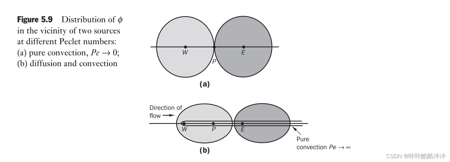
properties of discretisation schemes
conservation 守恒性
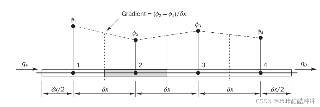
用纯扩散性方程分析:
(
Γ
ϕ
2
−
ϕ
1
δ
x
−
q
A
)
+
(
Γ
ϕ
3
−
ϕ
2
δ
x
−
Γ
ϕ
2
−
ϕ
1
δ
x
)
+
(
Γ
ϕ
4
−
ϕ
3
δ
x
−
Γ
ϕ
3
−
ϕ
2
δ
x
)
+
(
q
B
−
Γ
ϕ
4
−
ϕ
3
δ
x
)
=
q
B
−
q
A
(\Gamma\frac{\phi_2-\phi_1}{\delta x}-q_A)+(\Gamma\frac{\phi_3-\phi_2}{\delta x}-\Gamma\frac{\phi_2-\phi_1}{\delta x})+(\Gamma\frac{\phi_4-\phi_3}{\delta x}-\Gamma\frac{\phi_3-\phi_2}{\delta x})+(q_B-\Gamma\frac{\phi_4-\phi_3}{\delta x})=q_B-q_A
(Γδxϕ2−ϕ1−qA)+(Γδxϕ3−ϕ2−Γδxϕ2−ϕ1)+(Γδxϕ4−ϕ3−Γδxϕ3−ϕ2)+(qB−Γδxϕ4−ϕ3)=qB−qA
Boundedness 有界性
- 对角占优 diagonally dominant
- ϕ \phi ϕ应该在neighboring nods的值范围内
- 离散方程的所有系数应具有相同的符号
不过不符合以上条件,就可能越界 产生“wiggles”现象
example
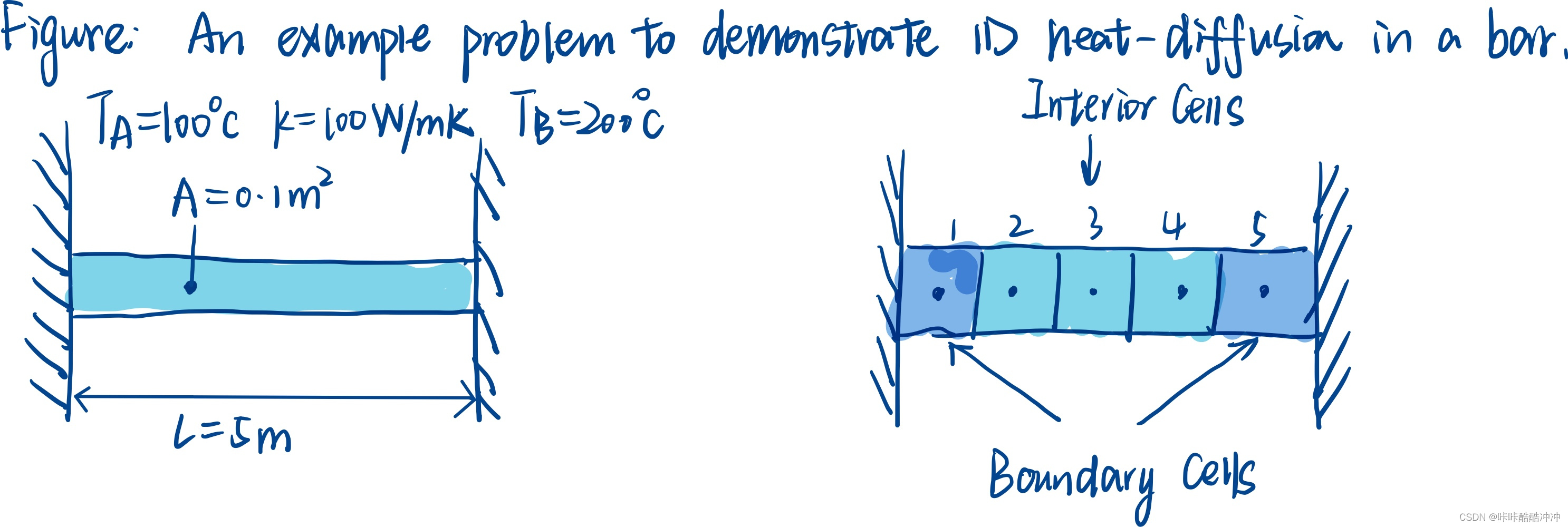
一维稳态扩散方程
d
d
x
(
k
d
T
d
x
)
+
S
=
0
\frac{d}{dx}(k\frac{dT}{dx})+S=0
dxd(kdxdT)+S=0
(
k
A
T
R
−
T
P
d
P
R
)
−
(
k
A
T
P
−
T
L
d
L
P
)
+
S
‾
V
=
0
(kA\frac{T_R-T_P}{d_{PR}})-(kA\frac{T_P-T_L}{d_{LP}})+\overline S V=0
(kAdPRTR−TP)−(kAdLPTP−TL)+SV=0
- 内部网格:
( k A d T d x ) r − ( k A d T d x ) l + S ‾ V = 0 (kA\frac{dT}{dx})_r-(kA\frac{dT}{dx})_l+\overline S V=0 (kAdxdT)r−(kAdxdT)l+SV=0
T P ( D l A l + D r A r + 0 ) = T L ( D l A l ) + T R ( D r A r ) + S ‾ V = 0 T_P(D_lA_l+D_rA_r+0)=T_L(D_lA_l)+T_R(D_rA_r)+\overline SV=0 TP(DlAl+DrAr+0)=TL(DlAl)+TR(DrAr)+SV=0 - 边界网格:
( k A d T d x ) r − ( k A d T d x ) l + S ‾ V = 0 (kA\frac{dT}{dx})_r-(kA\frac{dT}{dx})_l+\overline S V=0 (kAdxdT)r−(kAdxdT)l+SV=0
left
( d T d x ) l = T P − T A d L P / 2 (\frac{dT}{dx})_l=\frac{T_P-T_A}{d_{LP/2}} (dxdT)l=dLP/2TP−TA
( k A T R − T P d P R ) − ( k l T P − T A d L P / 2 ) + V ‾ = 0 (kA\frac{T_R-T_P}{d_{PR}})-(kl\frac{T_P-T_A}{d_{LP}/2})+\overline V=0 (kAdPRTR−TP)−(kldLP/2TP−TA)+V=0
T P ( 0 + D A + 2 D A ) = T L ( 0 ) + T R ( D A ) + T A ( 2 D A ) + S ‾ V T_P(0+DA+2DA)=T_L(0)+T_R(DA)+T_A(2DA)+\overline SV TP(0+DA+2DA)=TL(0)+TR(DA)+TA(2DA)+SV
right
T P ( D A + 0 + 2 D A ) = T L ( D l A l ) + T R ( 0 ) + T B ( 2 D A ) + S ‾ V T_P(DA+0+2DA)=T_L(D_lA_l)+T_R(0)+T_B(2DA)+\overline SV TP(DA+0+2DA)=TL(DlAl)+TR(0)+TB(2DA)+SV
- 分割网格
L c e l l = L N = 1 m L_cell=\frac{L}{N}=1m Lcell=NL=1m - 分配材料属性
D A = 10 ∗ 0.1 / 1 = 10 [ W / K ] DA=10*0.1/1=10[W/K] DA=10∗0.1/1=10[W/K]
S ‾ V = 1000 ∗ 0.1 ∗ 1 = 100 [ W ] \overline S V=1000*0.1*1=100[W] SV=1000∗0.1∗1=100[W] - 矩阵系数
A matrix:
  30.0  -10.0    0.0    0.0    0.0
 -10.0   20.0  -10.0    0.0    0.0
   0.0  -10.0   20.0  -10.0    0.0
   0.0    0.0  -10.0   20.0  -10.0
   0.0    0.0    0.0  -10.0   30.0

B vector:
2100.0
 100.0
 100.0
 100.0
4100.0
- 求解矩阵
T = A / B T=A/B T=A/B
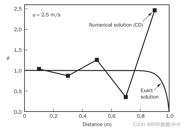
case2- wiggle-对流扩散
close all; clear; clc
%--------------------------------------------------------------------------
% User Inputs
%--------------------------------------------------------------------------
% Thermal Conductivity of the fluid (W/mK)
cond = 0.1;
% Specific heat capacity of the bar (J/Kg K)
cp = 1;
% Cross-sectional Area of the channel (m2)
area = 1;
% Length of the channel (m)
barLength = 1;
% Number of cells in the mesh
nCells = 5;
% Temperature at the left hand side of the channel (deg C)
tempLeft = 1;
% Temperature at the right hand side of the channel (deg C)
tempRight = 0;
% Heat source per unit volume (W/m3)
heatSourcePerVol = 0;
% Flow velocity (m/s)
flowVelocity = 2.5;
% Fluid Density (kg/m3)
fluidDensity = 1.0;
% Plot the data? ('true' / 'false')
plotOutput = 'true';
% Print the set up data? (table of coefficients and matrices)
printSetup = 'true';
% Print the solution output (the temperature vector)
printSolution = 'true';
% =========================================================================
% Code Begins Here
% =========================================================================
%--------------------------------------------------------------------------
% 1. Print messages
%--------------------------------------------------------------------------
fprintf('================================================\n');
fprintf('\n');
fprintf(' solve1DConvectionDiffusionEquationUpwind.m\n')
fprintf('\n')
fprintf(' - Fluid Mechanics 101\n')
fprintf(' - Author: Dr. Aidan Wimshurst\n')
fprintf(' - Contact: FluidMechanics101@gmail.com\n')
fprintf('\n')
fprintf(' [Exercise 1: Chapter 4]\n')
fprintf('================================================\n')
%--------------------------------------------------------------------------
% 2. Create the mesh of cells
%--------------------------------------------------------------------------
fprintf(' Creating Mesh ...\n');
fprintf('------------------------------------------------\n');
% Start by calculating the coordinates of the cell faces
xFaces = linspace(0, barLength, nCells+1);
% Calculate the coordinates of the cell centroids
xCentroids = 0.5*(xFaces(2:end) + xFaces(1:end-1));
% Calculate the length of each cell
cellLength = xFaces(2:end) - xFaces(1:end-1);
% Calculate the distance between cell centroids
dCentroids = xCentroids(2:end) - xCentroids(1:end-1);
% For the boundary cell on the left, the distance is double the distance
% from the cell centroid to the boundary face
dLeft = 2*(xCentroids(1) - xFaces(1));
% For the boundary cell on the right, the distance is double the distance from
% the cell centroid to the boundary cell face
dRight = 2*(xFaces(end) - xCentroids(end));
% Append these to the vector of distances
dCentroids = [dLeft, dCentroids, dRight];
% Compute the cell volume
cellVolumes = cellLength*area;
%--------------------------------------------------------------------------
% 2.0 Calculate the Matrix Coefficients
%--------------------------------------------------------------------------
fprintf(' Calculating Matrix Coefficients\n');
fprintf('------------------------------------------------\n');
% Diffusive flux per unit area
DA = area*cond./dCentroids;
% Convective flux
velocityVector = flowVelocity*ones(1, nCells+1);
densityVector = fluidDensity*ones(1, nCells+1);
F = densityVector.*velocityVector*area*cp;
% Evaluate the Peclet Number
Pe = F./DA;
% Calculate the source term Sp
Sp = zeros(1, nCells);
% Assign sources to the left and right hand boundaries
Sp(1) = -1.0*(2.0*DA(1) +F(1));
Sp(end) = -1.0*(2.0*DA(end) -F(end));
% Calculate the source term Su
Su = heatSourcePerVol*cellVolumes;
% Assign sources to the left and right hand boundaries
Su(1) = 3.5*tempLeft;
Su(end) = -3.5*tempRight;
% Left Coefficient (aL)
aL = DA(1:end-1) + (F(1:end-1)/2);
%Right Coefficient (aR)
aR = DA(2:end) + (-F(2:end)/2);
% Set the first element of aL to zero. It is a boundary face
aL(1) = 0;
% Set the last element of aR to zero. It is a boundary face
aR(end) = 0;
% Create the central coefficients
aP = aL + aR - Sp;
%--------------------------------------------------------------------------
% 3.0 Create the matrices
%--------------------------------------------------------------------------
fprintf(' Assembling Matrices\n');
fprintf('------------------------------------------------\n');
% Start by creating an empty A matrix and an empty B matrix
Amatrix = zeros(nCells, nCells);
BVector = zeros(nCells, 1);
% Populate the matrix one row at a time (i.e one cell at a time)
%
% NOTE: this method is deliberately inefficient for this problem
% but it is useful for learning purposes. We could populate the
% diagonals and the off-diagonals directly.
for i = 1:nCells
% Do the A matrix Coefficients
% Left boundary Cell
if (i == 1)
Amatrix(i, i) = aP(i);
Amatrix(i, i+1) = -1.0*aR(i);
% Right Boundary Cell
elseif(i == nCells)
Amatrix(i, i-1) = -1.0*aL(i);
Amatrix(i, i) = aP(i);
% Interior Cells
else
Amatrix(i, i-1) = -1.0*aL(i);
Amatrix(i, i) = aP(i);
Amatrix(i, i+1) = -1.0*aR(i);
end
% Do the B matrix coefficients
BVector(i) = Su(i);
end
%--------------------------------------------------------------------------
% 4.0 Print the setup
%--------------------------------------------------------------------------
if strcmp(printSetup, 'true')
fprintf(' Summary: Set Up\n')
fprintf('------------------------------------------------\n')
fprintf('aL: ')
for i = 1:nCells
fprintf('%6.1f ', aL(i));
end
fprintf('\n')
fprintf('aR: ')
for i = 1:nCells
fprintf('%6.1f ', aR(i));
end
fprintf('\n')
fprintf('aP: ')
for i = 1:nCells
fprintf('%6.1f ', aP(i));
end
fprintf('\n')
fprintf('Sp: ')
for i = 1:nCells
fprintf('%6.1f ', Sp(i));
end
fprintf('\n')
fprintf('Su: ')
for i = 1:nCells
fprintf('%6.1f ', Su(i));
end
fprintf('\n')
fprintf('Pe: ')
for i = 1:nCells+1
fprintf('%6.1f ', Pe(i));
end
fprintf('\n')
fprintf('A matrix:\n')
for i = 1:nCells
for j = 1:nCells
fprintf('%6.1f ', Amatrix(i, j));
end
fprintf('\n')
end
fprintf('B vector:\n')
for i = 1:nCells
fprintf('%6.1f\n', BVector(i));
end
fprintf('\n')
fprintf('------------------------------------------------\n')
end
%--------------------------------------------------------------------------
% 5.0 Solve the matrices
%--------------------------------------------------------------------------
fprintf(' Solving ...\n')
fprintf('------------------------------------------------\n')
% Use MATLAB's default linear algebra solver (AX = B)
Tvector = Amatrix \ BVector;
fprintf(' Equations Solved.\n')
fprintf('------------------------------------------------\n')
%--------------------------------------------------------------------------
% 6.0 Print the Solution
%--------------------------------------------------------------------------
if strcmp(printSolution, 'true')
fprintf(' Solution: Temperature Vector\n');
fprintf('------------------------------------------------\n');
fprintf('T vector:\n')
for i = 1:nCells
fprintf('%10.6f\n', Tvector(i));
end
fprintf('\n')
fprintf('------------------------------------------------\n')
end
%--------------------------------------------------------------------------
% 7.0 Plot the solution
%--------------------------------------------------------------------------
% Plot the data if desired
if strcmp(plotOutput,'true')
fprintf(' Plotting ...\n')
fprintf('------------------------------------------------\n')
% Append the boundary temperature values to the vector, so we can
% plot the complete solution
xPlotting = [xFaces(1), xCentroids, xFaces(end)];
temperaturePlotting = [tempLeft; Tvector; tempRight];
% Figure Size Parameters
figSizeXcm = 8.5;
aspectRatio = 4.0/3.0;
figSizeYcm = figSizeXcm / aspectRatio;
figSizeXpixels = figSizeXcm * 37.79527559055118;
figSizeYpixels = figSizeYcm * 37.79527559055118;
% Figure font, text and line widths
fontSize = 10;
fontChoice = 'Arial';
lineWidth = 1.0;
markerSize = 4;
% Colours for the line plots
colour1 = 'black';
colour2 = [0.0, 0.129, 0.2784];
% Adjust anchor for where figure shows up on screen (px)
x0 = 100;
y0 = 100;
fig1 = figure('Name', '1D Diffusion');
box on;
hold on;
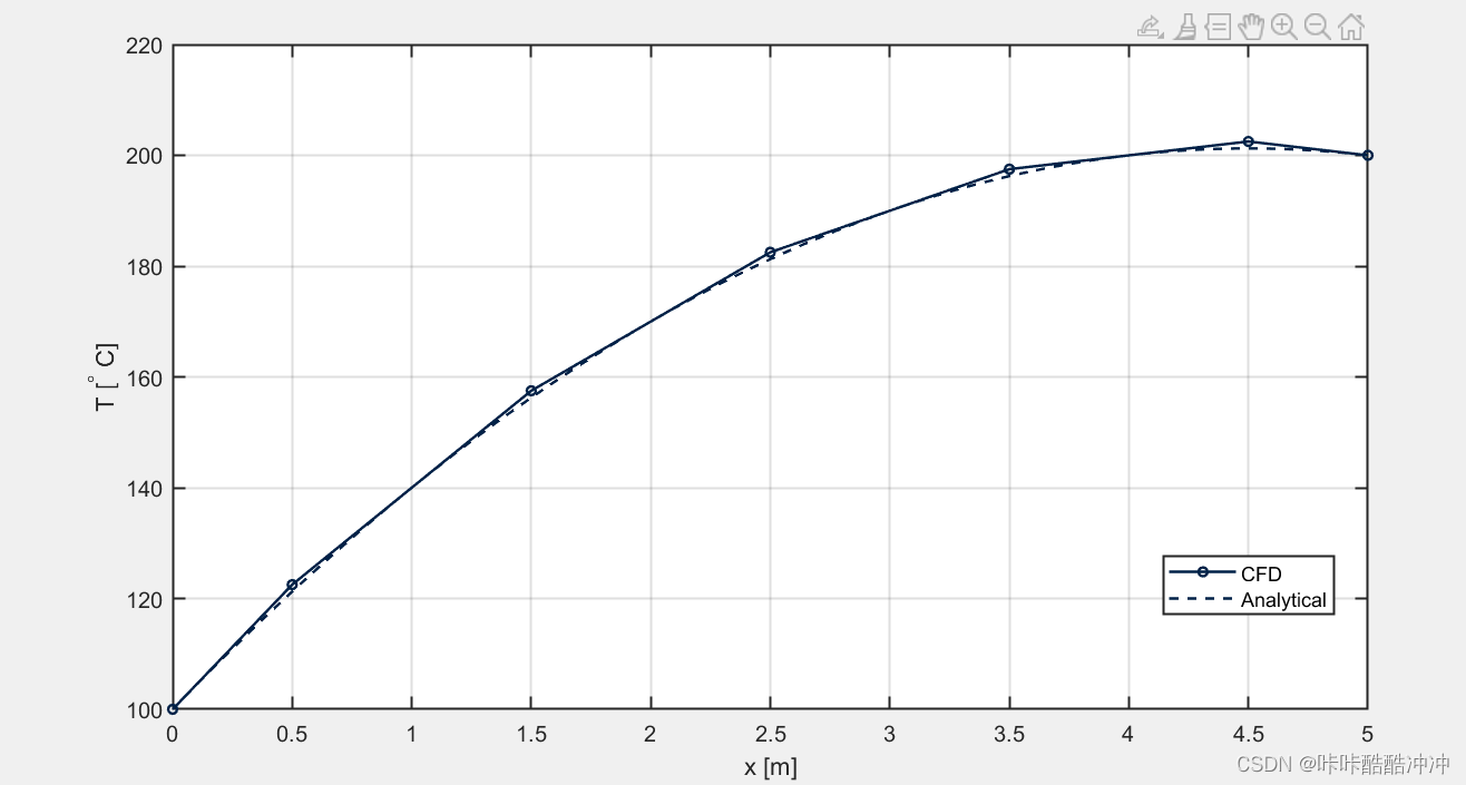
plot(xPlotting, temperaturePlotting, 'k-o', 'Color', colour2, ...
'MarkerSize', markerSize, 'linewidth', lineWidth + 0.2);
hold off;
xlabel('x [m]', 'FontSize', fontSize)
ylabel('T [^{\circ} C]', 'FontSize', fontSize)
grid on;
set(gca, 'fontsize', fontSize);
set(gca, 'linewidth', lineWidth);
set(gcf, 'position', [x0, y0, figSizeXpixels, figSizeYpixels]);
legend({'CFD'}, 'NumColumns', 1, 'Location', 'Best')
end
%==========================================================================
% END OF FILE
%==========================================================================
结果:
================================================
 Creating Mesh ...
------------------------------------------------
 Calculating Matrix Coefficients
------------------------------------------------
 Assembling Matrices
------------------------------------------------
 Summary: Set Up
------------------------------------------------
aL:    0.0    1.8    1.8    1.8    1.8
aR:   -0.8   -0.7   -0.7   -0.8    0.0
aP:    2.8    1.0    1.0    1.0    0.3
Sp:   -3.5    0.0    0.0    0.0    1.5
Su:    3.5    0.0    0.0    0.0   -0.0
Pe:    5.0    5.0    5.0    5.0    5.0    5.0
A matrix:
   2.8    0.8    0.0    0.0    0.0
  -1.8    1.0    0.7    0.0    0.0
   0.0   -1.8    1.0    0.7    0.0
   0.0    0.0   -1.8    1.0    0.8
   0.0    0.0    0.0   -1.8    0.3
B vector:
   3.5
   0.0
   0.0
   0.0
  -0.0

------------------------------------------------
 Solving ...
------------------------------------------------
 Equations Solved.
------------------------------------------------
 Solution: Temperature Vector
------------------------------------------------
T vector:
  1.035630
  0.869355
  1.257331
  0.352053
  2.464370

------------------------------------------------
 Plotting ...
------------------------------------------------
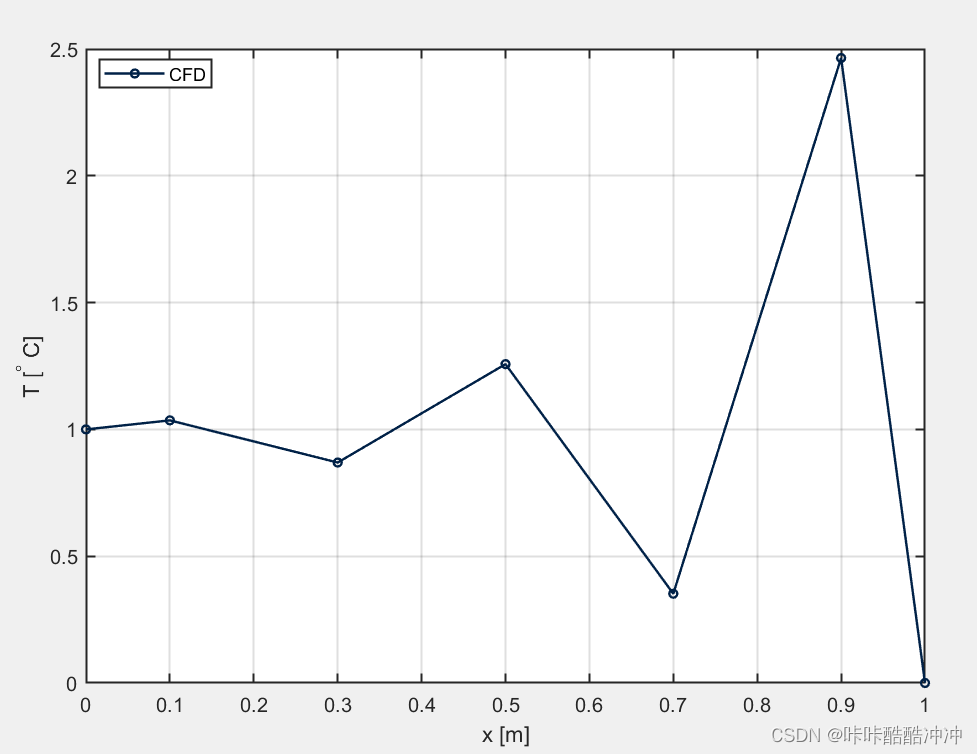
- CD方法计算,Pe数大(5)造成越界
参考:
- book-An Introduction to Computational Fluid Dynamics, The Finite Volume Method
================================================

   solve1DConvectionDiffusionEquationUpwind.m

 - Fluid Mechanics 101
 - Author: Dr. Aidan Wimshurst
 - Contact: FluidMechanics101@gmail.com

 [Exercise 1: Chapter 4]
Transportiveness 输运性
Accuracy 精度
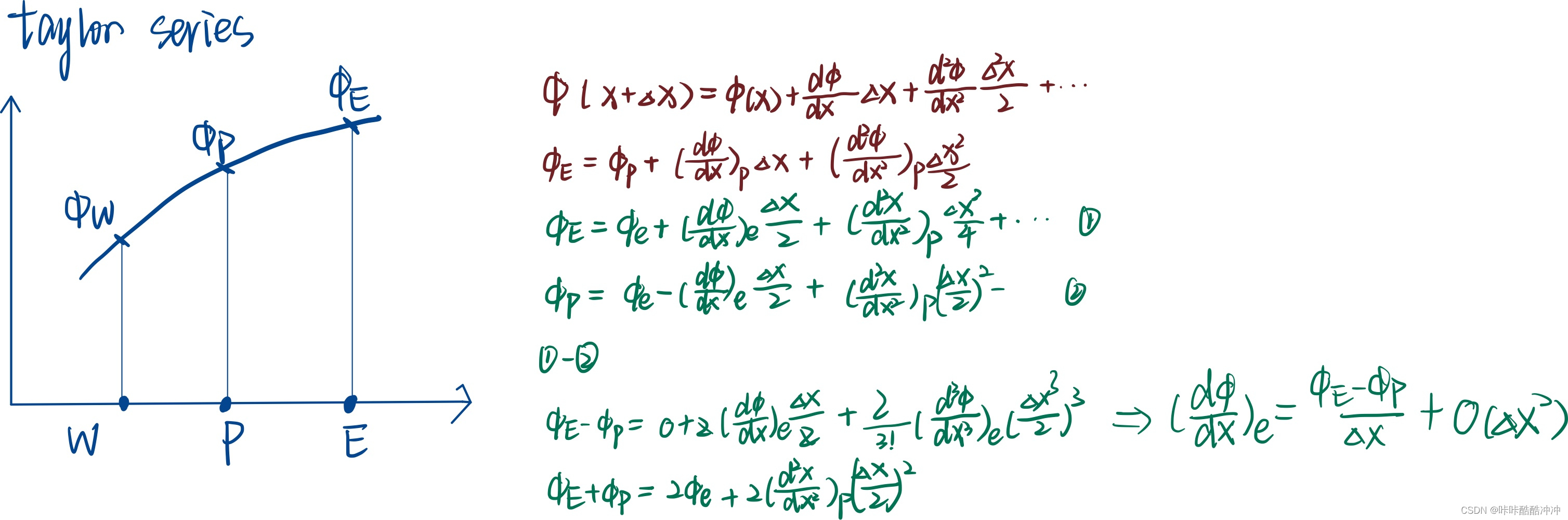
QUICK格式3阶
ϕ e = 3 8 ϕ E + 6 8 ϕ P − 1 8 ϕ W \phi_e=\frac{3}{8}\phi_E+\frac{6}{8}\phi_P- \frac{1}{8} \phi_W ϕe=83ϕE+86ϕP−81ϕW
- 用了三个点,三阶格式
- 迎风格式,非常稳定的格式,不会越界,守恒,一阶格式,会带来smear现象。
- CD,可能会导致越界,二阶
- 二阶迎风格式
- QUICK,三阶格式


 1030
1030


 被折叠的 条评论
为什么被折叠?
被折叠的 条评论
为什么被折叠?
 到【灌水乐园】发言


