为什么L1正则项会产生稀疏解

Consider the vector $\vec{x}=(1,\varepsilon)\in\mathbb{R}^2$ where $\varepsilon>0$ is small. The $l_1$ and $l_2$ norms of $\vec{x}$, respectively, are given by

$$||\vec{x}||_1 = 1+\varepsilon,\ \ ||\vec{x}||_2^2 = 1+\varepsilon^2$$

Now say that, as part of some regularization procedure, we are going to reduce the magnitude of one of the elements of $\vec{x}$ by $\delta\leq\varepsilon$. If we change $x_1$ to $1-\delta$, the resulting norms are

$$||\vec{x}-(\delta,0)||_1 = 1-\delta+\varepsilon,\ \ ||\vec{x}-(\delta,0)||_2^2 = 1-2\delta+\delta^2+\varepsilon^2$$

On the other hand, reducing $x_2$ by $\delta$ gives norms

$$||\vec{x}-(0,\delta)||_1 = 1-\delta+\varepsilon,\ \ ||\vec{x}-(0,\delta)||_2^2 = 1-2\varepsilon\delta+\delta^2+\varepsilon^2$$

The thing to notice here is that, for an $l_2$ penalty, regularizing the larger term $x_1$ results in a much greater reduction in norm than doing so to the smaller term $x_2\approx 0$. For the $l_1$ penalty, however, the reduction is the same. Thus, when penalizing a model using the $l_2$ norm, it is highly unlikely that anything will ever be set to zero, since the reduction in norm going from $\varepsilon$ to $0$ is almost nonexistent when $\varepsilon$ is small. On the other hand, the reduction in $l_1$ norm is always equal to $\delta$, regardless of the quantity being penalized.

Another way to think of it: it’s not so much that $l_1$ penalties encourage sparsity, but that $l_2$ penalties in some sense discourage sparsity by yielding diminishing returns as elements are moved closer to zero.

an $l_\alpha$ penalty for any $\alpha\leq1$ will also induce sparsity, but you see those less often in practice (probably because they’re non-convex). If you really just want sparsity then an $l_0$ penalty (proportional to the number of non-zero entries) is the way to go, it just so happens that it’s a bit of a nightmare to work with.

Yes - that’s correct. There are many norms that lead to sparsity (e.g., as you mentioned, any Lp norm with p <= 1). In general, any norm with a sharp corner at zero induces sparsity. So, going back to the original question - the L1 norm induces sparsity by having a discontinuous gradient at zero (and any other penalty with this property will do so too)

Have a look on figure 3.11 (page 71) of The elements of statistical learning. It shows the position of a unconstrained $\hat \beta$ that minimizes the squared error function, the ellipses showing the levels of the square error function, and where are the $\hat \beta$ subject to constraints $\ell_1 (\hat \beta) < t$ and $\ell_2 (\hat \beta) < t$.

This will allow you to understand very geometrically that subject to the $\ell_1$ constraint, you get some null components. This is basically because the $\ell_1$ ball $\{ x : \ell_1(x) \le 1\}$ has “edges” on the axes.

More generally, this book is a good reference on this subject: both rigorous and well illustrated, great explanations.

I think your second paragraph is a key… at least for my intuition: an l1 “ball” is more like a diamond that’s spikey along the axes, which means that a hyperplane constrained to hit it is more likely to have a zero on the axes.

Yes, I use to imagine the optimization process as the movement of a point submitted to two forces : attraction towards the unconstrained $\hat \beta$ thanks to the squared error function, attraction towards 0 thaks to the $\ell_1$ or $\ell_2$ norm. Here, the “geometry” of this attraction force changes the behavior of the point. If you fix a small $\ell_1$ or $\ell_2$ ball in which it can freely move, it will slide on the border of the ball, in order to go near to $\hat \beta$. The result is shown on the illustration in the aforementionned book.

With a sparse model, we think of a model where many of the weights are 0. Let us therefore reason about how L1-regularization is more likely to create 0-weights.

Consider a model consisting of the weights $(w_1, w_2, \dots, w_m)$.

With L1 regularization, you penalize the model by a loss function $L_1(w)$ = $\Sigma_i |w_i|$.

With L2-regularization, you penalize the model by a loss function $L_2(w)$ = $\frac{1}{2} \Sigma_i w_i^2$

If using gradient descent, you will iteratively make the weights change in the opposite direction of the gradient with a step size $\eta$. Let us look at the gradients:

$\frac{dL_1(w)}{dw} = sign(w)$, where $sign(w) = (\frac{w_1}{|w_1|}, \frac{w_1}{|w_1|}, \dots, \frac{w_1}{|w_m|})$

$\frac{dL_2(w)}{dw} = w$

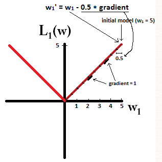
If we plot the loss function and it’s derivative for a model consisting of just a single parameter, it looks like this for L1:

Notice that for $L_1$, the gradient is either 1 or -1, except for when $w_1 = 0$. That means that L1-regularization will move any weight towards 0 with the same step size, regardless the weight’s value. In contrast, you can see that the $L_2$ gradient is linearly decreasing towards 0 as the weight goes towards 0. Therefore, L2-regularization will also move any weight towards 0, but it will take smaller and smaller steps as a weight approaches 0.

Try to imagine that you start with a model with $w_1 = 5$ and using $\eta = \frac{1}{2}$. In the following picture, you can see how gradient descent using L1-regularization makes 10 of the updates $w_1 := w_1 - \eta \cdot \frac{dL_1(w)}{dw} = w_1 - 0.5 \cdot 1$, until reaching a model with $w_1 = 0$:

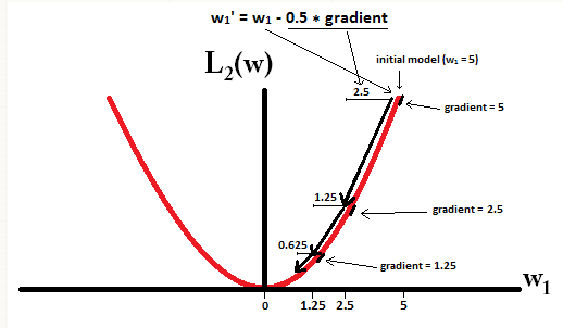
In constrast, with L2-regularization where $\eta = \frac{1}{2}$, the gradient is $w_1$, causing every step to be only halfway towards 0. That is we make the update $w_1 := w_1 - \eta \cdot \frac{dL_1(w)}{dw} = w_1 - 0.5 \cdot w_1$ Therefore, the model never reaches a weight of 0, regardless of how many steps we take:

Note that L2-regularization can make a weight reach zero if the step size $\eta$ is so high that it reaches zero or beyond in a single step. However, the loss function will also consist of a term measuring the error of the model with the respect to the given weights, and that term will also affect the gradient and hence the change in weights. However, what is shown in this example is just how the two types of regularization contribute to a change in weights.