


原理部分
KNN算法原理
参考博客:https://blog.csdn.net/jmydream/article/details/8644004
kNN算法则是从训练集中找到和新数据最接近的k条记录,然后根据他们的主要分类来决定新数据的类别。该算法涉及3个主要因素:训练集、距离或相似的衡量、k的大小。

kNN算法的指导思想是“近朱者赤,近墨者黑”,由你的邻居来推断出你的类别。
计算步骤:
1)算距离:给定测试对象,计算它与训练集中的每个对象的距离
2)找邻居:圈定距离最近的k个训练对象,作为测试对象的近邻
3)做分类:根据这k个近邻归属的主要类别,来对测试对象分类
2、距离或相似度的衡量
什么是合适的距离衡量?距离越近应该意味着这两个点属于一个分类的可能性越大。
觉的距离衡量包括欧式距离、夹角余弦等。
对于文本分类来说,使用余弦(cosine)来计算相似度就比欧式(Euclidean)距离更合适。
3、类别的判定
投票决定:少数服从多数,近邻中哪个类别的点最多就分为该类。
加权投票法:根据距离的远近,对近邻的投票进行加权,距离越近则权重越大(权重为距离平方的倒数)
优缺点
1、优点
简单,易于理解,易于实现,无需估计参数,无需训练
适合对稀有事件进行分类(例如当流失率很低时,比如低于0.5%,构造流失预测模型)
特别适合于多分类问题(multi-modal,对象具有多个类别标签),例如根据基因特征来判断其功能分类,kNN比SVM的表现要好
2、缺点
懒惰算法,对测试样本分类时的计算量大,内存开销大,评分慢
可解释性较差,无法给出决策树那样的规则。
Dense-sift(稠密SIFT)原理
图像检索总是用SIFT(利用了检测子)
大多数情况下我们并没有训练样本。因此,我们需要利用人的经验过滤区分性低的点(除此之外还引入了IDF进一步加权)。因此,大部分检索问题都利用了检测子,而不是密集采样。
图像识别问题大多用Dense-SIFT
Dense-SIFT在非深度学习的模型中,常常是特征提取的第一步
对于图像识别问题来说,由于有充足的训练样本(正负样本均充足)。通过对训练样本的学习,我们会学习一个分类器。
总而言之,当研究目标是对同样的物体或者场景寻找对应关系(correspondence)时, SIFT更好。而研究目标是图像表示或者场景理解时,Dense SIFT更好,因为即使密集采样的区域不能够被准确匹配,这块区域也包含了表达图像内容的信息。

代码实现
KNN算法实现
实现最基本的 KNN算法
class KnnClassifier(object):

    def __init__(self,labels,samples):
        """ Initialize classifier with training data.使用训练数据初始化分类器  """

        self.labels = labels
        self.samples = samples

    def classify(self,point,k=3):
        """ Classify a point against k nearest
            in the training data, return label.
             在训练数据上采用 k 近邻分类,并返回标记
        """

        # compute distance to all training points 计算所有训练数据点的距离
        dist = array([L2dist(point,s) for s in self.samples])

        # sort them 对它们进行排序
        ndx = dist.argsort()

        # use dictionary to store the k nearest   用字典存储 k 近邻
        votes = {}
        for i in range(k):
            label = self.labels[ndx[i]]
            votes.setdefault(label,0)
            votes[label] += 1

        return max(votes, key=lambda x: votes.get(x))
定义一个类并用训练数据初始化非常简单 ; 每次想对某些东西进行分类时,用 KNN 方法,我们就没有必要存储并将训练数据作为参数来传递。用一个字典来存储邻近标记,我们便可以用文本字符串或数字来表示标记。在这个例子中,我们用欧式距 离 (L2) 进行度量。
我们首先建立一些简单的二维示例数据集来说明并可视化分类器的工作原理,下面的脚本将创建两个不同的二维点集,每个点集有两类,用 Pickle 模块来保存创建的数据:
data.py
# -*- coding: utf-8 -*-
from numpy.random import randn
import pickle
from pylab import *

# create sample data of 2D points
# 创建二维样本数据
n = 200
# two normal distributions
# 两个正态分布数据集
class_1 = 0.2 * randn(n,2)
class_2 = 1.6 * randn(n,2) + array([5,1])
labels = hstack((ones(n),-ones(n)))
# save with Pickle
# 用 Pickle 模块保存
#with open('points_normal.pkl', 'w') as f:
with open('points_normal_test.pkl', 'wb') as f:
    pickle.dump(class_1,f)
    pickle.dump(class_2,f)
    pickle.dump(labels,f)
# normal distribution and ring around it
# 正态分布,并使数据成环绕状分布
print ("save OK!")
class_1 = 0.6 * randn(n,2)
r = 0.8 * randn(n,1) + 5
angle = 2*pi * randn(n,1)
class_2 = hstack((r*cos(angle),r*sin(angle)))
labels = hstack((ones(n),-ones(n)))
# save with Pickle
# 用 Pickle 保存
#with open('points_ring.pkl', 'w') as f:
with open('points_ring_test.pkl', 'wb') as f:
    pickle.dump(class_1,f)
    pickle.dump(class_2,f)
    pickle.dump(labels,f)

print ("save OK!")
kNN分类器:
# -*- coding: utf-8 -*-
import pickle
from pylab import *
from PCV.classifiers import knn
from PCV.tools import imtools

pklist=['points_normal.pkl','points_ring.pkl']

figure()

# load 2D points using Pickle
# 用Pickle模块来创建一个kNN分类器
for i, pklfile in enumerate(pklist):
    with open(pklfile, 'rb') as f:
        class_1 = pickle.load(f)
        class_2 = pickle.load(f)
        labels = pickle.load(f)
    # load test data using Pickle
    # 用Pickle模块载入测试数据
    with open(pklfile[:-4]+'_test.pkl', 'rb') as f:
        class_1 = pickle.load(f)
        class_2 = pickle.load(f)
        labels = pickle.load(f)

    model = knn.KnnClassifier(labels,vstack((class_1,class_2)))
    # test on the first point(数据集的第一个点)
    print (model.classify(class_1[0]))

    #define function for plotting
    def classify(x,y,model=model):
        return array([model.classify([xx,yy]) for (xx,yy) in zip(x,y)])

    # lot the classification boundary
    subplot(1,2,i+1)
    imtools.plot_2D_boundary([-6,6,-6,6],[class_1,class_2],classify,[1,-1])
    titlename=pklfile[:-4]
    title(titlename)
show()
可视化分类方法
def plot_2D_boundary(plot_range,points,decisionfcn,labels,values=[0]):
    """    Plot_range is (xmin,xmax,ymin,ymax), points is a list
        of class points, decisionfcn is a funtion to evaluate,
        labels is a list of labels that decisionfcn returns for each class,
        values is a list of decision contours to show.
        Plot_range 为(xmin,xmax,ymin,ymax),points 是类数据点列表,    decisionfcn 是评估函数,labels 是函数 decidionfcn 关于每个类返回的标记列表
        """
    # 在一个网格上进行评估,并画出决策函数的边界
    clist = ['b','r','g','k','m','y'] # colors for the classes

    # evaluate on a grid and plot contour of decision function
    x = arange(plot_range[0],plot_range[1],.1)
    y = arange(plot_range[2],plot_range[3],.1)
    xx,yy = meshgrid(x,y)# 用 meshgrid() 函数在一个网格上进行预测 沿着x轴,y轴 一个个点,一个个位置找
    xxx,yyy = xx.flatten(),yy.flatten() # lists of x,y in grid # 网格中的 x,y 坐标点列表
    zz = array(decisionfcn(xxx,yyy))
    zz = zz.reshape(xx.shape)
    # plot contour(s) at values
    # 以 values 画出边界
    contour(xx,yy,zz,values)
    # 对于每类,用 * 画出分类正确的点,用 o 画出分类不正确的点
    # for each class, plot the points with '*' for correct, 'o' for incorrect
    for i in range(len(points)):
        d = decisionfcn(points[i][:,0],points[i][:,1])
        correct_ndx = labels[i]==d
        incorrect_ndx = labels[i]!=d
        plot(points[i][correct_ndx,0],points[i][correct_ndx,1],'*',color=clist[i])
        plot(points[i][incorrect_ndx,0],points[i][incorrect_ndx,1],'o',color=clist[i])

    axis('equal')
运行结果:
*形-分类正确的点 、o 形-分类不正确的点
n=200
n=400
结果分析:
在数据数量不同的情况下,分类结果没有太大差别,说明KNN算法是一种适应度较好的算法。


稠密SIFT可视化
稠密 SIFT 特征向量。
在整幅图像上用一个规则的网格应用 SIFT 描述子可以得到稠密 SIFT 的表示形式
dsift.py
from PIL import Image
from numpy import *
import os

from PCV.localdescriptors import sift


def process_image_dsift(imagename,resultname,size=20,steps=10,force_orientation=False,resize=None):
    """ Process an image with densely sampled SIFT descriptors
        and save the results in a file. Optional input: size of features,
        steps between locations, forcing computation of descriptor orientation
        (False means all are oriented upwards), tuple for resizing the image."""

    im = Image.open(imagename).convert('L')
    if resize!=None:
        im = im.resize(resize)
    m,n = im.size

    if imagename[-3:] != 'pgm':
        #create a pgm file
        im.save('tmp.pgm')
        imagename = 'tmp.pgm'

    # create frames and save to temporary file
    scale = size/3.0
    x,y = meshgrid(range(steps,m,steps),range(steps,n,steps))
    xx,yy = x.flatten(),y.flatten()
    frame = array([xx,yy,scale*ones(xx.shape[0]),zeros(xx.shape[0])])
    savetxt('tmp.frame',frame.T,fmt='%03.3f')

    path = os.path.abspath(os.path.join(os.path.dirname("__file__"),os.path.pardir))
    path = path + "\\ch8\\win32vlfeat\\sift.exe "
    print(path)

    if force_orientation:
        cmmd = str("sift " + imagename + " --output=" + resultname + " --read-frames=tmp.frame --orientations")
    else:
        cmmd = str("sift " + imagename + " --output=" + resultname + " --read-frames=tmp.frame")
    os.system(cmmd)
    os.system(cmmd)
    print(cmmd)
    print ('@ processed', imagename, 'to', resultname)
稠密sift可视化
# -*- coding: utf-8 -*-
from PCV.localdescriptors import sift, dsift
from pylab import  *
from PIL import Image

dsift.process_image_dsift('gesture/qqq.jpg','qqq.dsift',90,40,True)
l,d = sift.read_features_from_file('qqq.dsift')
im = array(Image.open('gesture/qqq.jpg'))
sift.plot_features(im,l,True)
title('dense SIFT')
show()
当
dsift.process_image_dsift(‘gesture/qqq.jpg’,‘qqq.dsift’,90,40,True)

当
dsift.process_image_dsift(‘gesture/qqq.jpg’,‘qqq.dsift’,10,10,True)


图像分类:手势识别 实现
手势识别
# -*- coding: utf-8 -*-
from PCV.localdescriptors import dsift
import os
from PCV.localdescriptors import sift
from pylab import *
from PCV.classifiers import knn
def get_imagelist(path):
""" Returns a list of filenames for
all jpg images in a directory. """
return [os.path.join(path,f) for f in os.listdir(path) if f.endswith('.ppm')]
def read_gesture_features_labels(path):
# create list of all files ending in .dsift
featlist = [os.path.join(path,f) for f in os.listdir(path) if f.endswith('.dsift')]
# read the features
features = []
for featfile in featlist:
l,d = sift.read_features_from_file(featfile)
features.append(d.flatten())
features = array(features)
# create labels
labels = [featfile.split('/')[-1][0] for featfile in featlist]
return features,array(labels)
def print_confusion(res,labels,classnames):
n = len(classnames)
# confusion matrix
class_ind = dict([(classnames[i],i) for i in range(n)])
confuse = zeros((n,n))
for i in range(len(test_labels)):
confuse[class_ind[res[i]],class_ind[test_labels[i]]] += 1
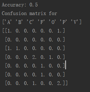
print ('Confusion matrix for')
print (classnames)
print (confuse)
filelist_train = get_imagelist('gesture/train')
filelist_test = get_imagelist('gesture/test1')
imlist=filelist_train+filelist_test
# process images at fixed size (50,50)
for filename in imlist:
featfile = filename[:-3]+'dsift'
dsift.process_image_dsift(filename,featfile,10,5,resize=(50,50))
features,labels = read_gesture_features_labels('gesture/train/')
test_features,test_labels = read_gesture_features_labels('gesture/test/')
classnames = unique(labels)
# test kNN
k = 1
knn_classifier = knn.KnnClassifier(labels,features)
res = array([knn_classifier.classify(test_features[i],k) for i in
range(len(test_labels))])
# accuracy
acc = sum(1.0*(res==test_labels)) / len(test_labels)
print ('Accuracy:', acc)
print_confusion(res,test_labels,classnames)
运行结果:
静态手势(Static Hand Posture)数据库结果:
训练集图片(自己拍摄):
test与train数据集完全相同:
正确率为100%


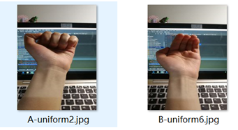
test与train数据集完全不同
情况1:
A手势与B手势与训练集姿势相反
放到静态手势(Static Hand Posture)数据库
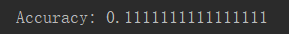
情况2:
A手势与B手势与训练集姿势相同
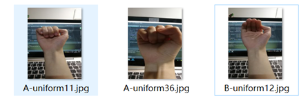
得到的正确率小幅上升
放到静态手势(Static Hand Posture)数据库
实验分析:
在进行图片识别时,KNN算法对图片的识别敏感。
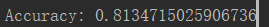
在训练集大的情况下,正确率可以达到81%。
在训练集小的情况下,正确率可以达到50%。
在静态手势(Static Hand Posture)数据库下,陌生场景下的手势正确率只能达到10%,
但是保持稳定状态。
从一方面,这说明,训练集过小,容易造成数据过拟合的问题
从另一方面,对不是很明显的手势区别也可以判断,分类敏感。
问题解决
问题1:.dsift文件无法正常生成
解决:
dsift.py 中保存时改成如下形式
if force_orientation:
    cmmd = str("sift " + imagename + " --output=" + resultname + " --read-frames=tmp.frame --orientations")
else:
    cmmd = str("sift " + imagename + " --output=" + resultname + " --read-frames=tmp.frame")
os.system(cmmd)
问题2:
报错:ValueError: operands could not be broadcast together with shapes (7296,) (7424,)
原因,两个数组的维度不匹配
解决方法:
knn.py
def L2dist(p1,p2):
    # print(len(p1))
    for i in range(7000):
        k=p1[i]-p2[i]
    # return sqrt( sum( (p1-p2)**2) )
    return sqrt( sum( k**2) )
PS:
读取一个文件夹的内容
imlist = imtools.get_imlist(‘gesture/test1/’)


 1035
1035


 被折叠的 条评论
为什么被折叠?
被折叠的 条评论
为什么被折叠?
 到【灌水乐园】发言


