吴恩达深度学习_2_Week3超参数调参、Batch正则化和程序框架(2)

最新推荐文章于 2024-05-21 23:36:04 发布

C夹夹

最新推荐文章于 2024-05-21 23:36:04 发布

阅读量47

点赞数

分类专栏：吴恩达深度学习文章标签：深度学习神经网络

本文链接：https://blog.csdn.net/zxy0000zxy/article/details/134320904

版权

吴恩达深度学习专栏收录该内容

23 篇文章 1 订阅

订阅专栏

Tensorflow_Tutorial

在TensorFlow中完成以下任务：
1、初始化变量
2、开启自己的会话
3、训练算法
4、实现神经网络

第二门课：改善深层神经网络：超参数调参、正则化以及优化
第三周：超参数调参、Batch正则化和程序框架

一、探索TensorFlow库

import math
import numpy as np
import h5py
import matplotlib.pyplot as plt
import tensorflow as tf
from tensorflow.python.framework import ops
from tf_utils import load_dataset, random_mini_batches, convert_to_one_hot, predict

np.random.seed(1)

示例：计算一个训练样本的损失

y_hat = tf.constant(36, name='y_hat')            # Define y_hat constant. Set to 36.
y = tf.constant(39, name='y')                    # Define y. Set to 39

loss = tf.Variable((y - y_hat)**2, name='loss')  # Create a variable for the loss

init = tf.global_variables_initializer()         # When init is run later (session.run(init)),
                                                 # the loss variable will be initialized and ready to be computed
with tf.Session() as session:                    # Create a session and print the output
    session.run(init)                            # Initializes the variables
    print(session.run(loss))                     # Prints the loss

在TensorFlow中编写和运行程序的步骤如下：
1、创建尚未执行/计算的张量（变量）。
2、在这些张量之间编写操作。
3、初始化张量。
4、创建一个会话（Session）。
5、运行会话。这将运行上面编写的操作。
因此，当为损失创建一个变量时，只是将损失定义为其他量的函数，但没有评估其值。要评估它，我们必须运行init=tf.global_variables_initializer()。这将初始化损失变量，在最后一行中，最终能够评估损失的值并打印出来。

a = tf.constant(2)
b = tf.constant(10)
c = tf.multiply(a,b)
print(c)

正如预期的那样，看不到20！得到的是一个张量，表示结果是一个没有形状属性的张量，类型为“int32”。所做的只是将其放入“计算图”中，但尚未运行此计算。为了实际上将这两个数字相乘，需要创建一个会话（Session）并运行它。

sess = tf.Session()
print(sess.run(c))

总结：记住要初始化的变量，创建一个会话并在会话中运行操作。

占位符是一个对象，其值只能在稍后指定。要为占位符指定值，可以使用“feed字典”（feed_dict变量）传递值。在下面的示例中，为x创建了一个占位符，能够在运行会话时稍后传入一个数字。

# Change the value of x in the feed_dict

x = tf.placeholder(tf.int64, name = 'x')
print(sess.run(2 * x, feed_dict = {x: 3}))
sess.close()

首次定义x时，无需为其指定值。占位符只是一个变量，将在运行会话时稍后为其赋值。在运行会话时，向这些占位符提供数据。
下面是发生的情况：当指定计算所需的操作时，正在告诉TensorFlow如何构建计算图。计算图中可以有一些占位符，将在稍后指定其值。最后，当运行会话时，正在告诉TensorFlow执行计算图。

1、线性函数

练习：计算𝑊𝑋+𝑏，其中𝑊、𝑋和𝑏是从随机正态分布中抽取的。W的形状为(4, 3)，X的形状为(3, 1)，b的形状为(4, 1)。
示例：如何定义一个具有形状(3, 1)的常量X：X = tf.constant(np.random.randn(3, 1), name=“X”)
tf.matmul(…) ：执行矩阵乘法
tf.add(…) ：执行加法
np.random.randn(…) ：随机初始化

实现线性函数：
初始化W为形状为(4, 3)的随机张量
初始化X为形状为(3, 1)的随机张量
初始化b为形状为(4, 1)的随机张量
返回：
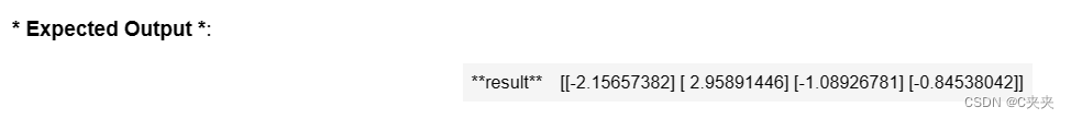
result：运行会话计算 Y = WX + b 的结果

def linear_function():
    np.random.seed(1)
    
    X = tf.constant(np.random.randn(3,1), name = "X")
    W = tf.constant(np.random.randn(4,3), name = "W")
    b = tf.constant(np.random.randn(4,1), name  = "b")
    Y = tf.add(tf.matmul(W, X), b)
    
    # 使用tf.Session()创建会话，并使用sess.run(...)在要计算的变量上运行它。
    sess = tf.Session()
    result = sess.run(Y)
    # 关闭session 
    sess.close()
    return result
 print( "result = " + str(linear_function()))

在这里插入图片描述

2、计算sigmoid激活函数

TensorFlow提供了许多常用的神经网络函数，如tf.sigmoid和tf.softmax。在这个练习中，计算输入的sigmoid函数。
使用一个占位符变量x来完成这个练习。在运行会话时，应该使用feed字典来传入输入z。
需要：(i) 创建一个占位符x，(ii) 定义计算sigmoid函数所需的操作，使用tf.sigmoid，然后 (iii) 运行会话。
练习：在下面实现sigmoid函数。可以使用以下方法：
tf.placeholder(tf.float32, name=“…”)
tf.sigmoid(…)
sess.run(…, feed_dict={x: z})
请注意，有两种在TensorFlow中创建和使用会话的典型方式：

# Method 1:
sess = tf.Session()
# Run the variables initialization (if needed), run the operations
result = sess.run(..., feed_dict = {...})
sess.close() # Close the session

# Method 2:
with tf.Session() as sess: 
    # run the variables initialization (if needed), run the operations
    result = sess.run(..., feed_dict = {...})
    # This takes care of closing the session for you :)

计算z的sigmoid函数。
参数：z：输入值，标量或向量
返回：result：z的sigmoid值

def sigmoid(z):
   
    # Create a placeholder for x. Name it 'x'.   
    x = tf.placeholder(tf.float32, name = "x")    
    # compute sigmoid(x)
    sigmoid = tf.sigmoid(x)
    
    # Create a session, and run it. Please use the method 2 explained above. 
    # You should use a feed_dict to pass z's value to x. 
    with tf.Session() as sess:
        # Run session and call the output "result"
         result = sess.run(sigmoid, feed_dict = {x:z})    
    return result
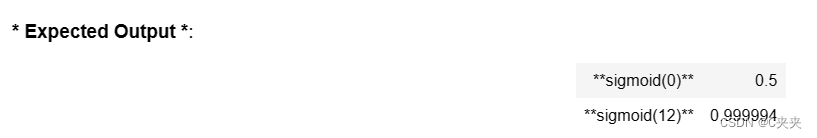
print ("sigmoid(0) = " + str(sigmoid(0)))
print ("sigmoid(12) = " + str(sigmoid(12)))

在这里插入图片描述
总结：
1、创建占位符（placeholders）
2、指定对应于要计算的操作的计算图（computation graph）
3、创建会话（session）
4、运行会话，如果需要指定占位符变量的值，可以使用feed字典（feed dictionary）

3、计算代价

在这里插入图片描述
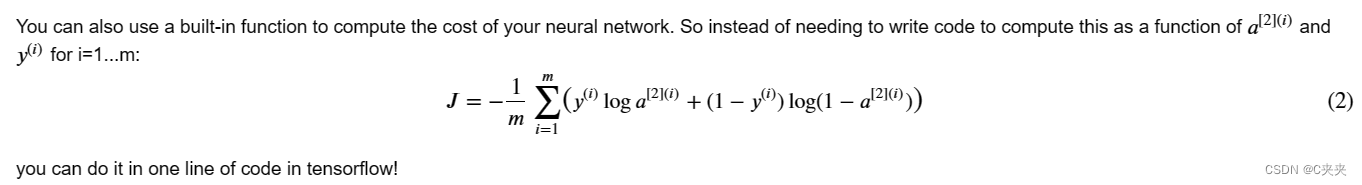
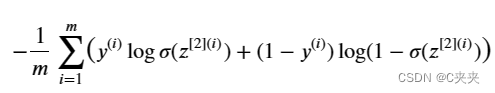
练习：实现交叉熵损失函数。使用的函数是：tf.nn.sigmoid_cross_entropy_with_logits(logits=…, labels=…)
应该输入z，计算sigmoid函数（得到a），然后计算交叉熵损失𝐽。
所有这些可以通过一次调用tf.nn.sigmoid_cross_entropy_with_logits来完成，该函数会计算交叉熵损失。
在这里插入图片描述

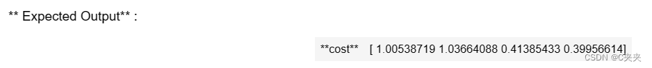
使用sigmoid交叉熵计算成本。
参数：
logits：包含z的向量，是最后一个线性单元的输出（在最终的sigmoid激活之前）
labels：标签y的向量（1或0）
注意：称之为“z”和“y”的东西在TensorFlow文档中分别称为“logits”和“labels”。因此，logits将作为z的输入，labels将作为y的输入。
返回：
cost：运行成本的会话（公式（2））

def cost(logits, labels):  
    # Create the placeholders for "logits" (z) and "labels" (y) (approx. 2 lines)
    z = tf.placeholder(tf.float32, name = "z")
    y = tf.placeholder(tf.float32, name = "y")
    
    # Use the loss function (approx. 1 line)
    cost = tf.nn.sigmoid_cross_entropy_with_logits(logits = z, labels = y)
    
    # Create a session (approx. 1 line). See method 1 above.
    sess = tf.Session()
  
    # Run the session (approx. 1 line).
    cost = sess.run(cost, feed_dict = {z:logits, y:labels})
   
    # Close the session (approx. 1 line). See method 1 above.
     sess.close()
     return cost
logits = sigmoid(np.array([0.2,0.4,0.7,0.9]))
cost = cost(logits, np.array([0,0,1,1]))
print ("cost = " + str(cost))

在这里插入图片描述

4、使用一位有效编码（One Hot Encoding）

在深度学习中，经常会有一个y向量，其中的数字范围是从0到C-1，其中C是类别的数量。例如，如果C是4，那么可能有以下y向量，您需要将其转换如下：
在这里插入图片描述
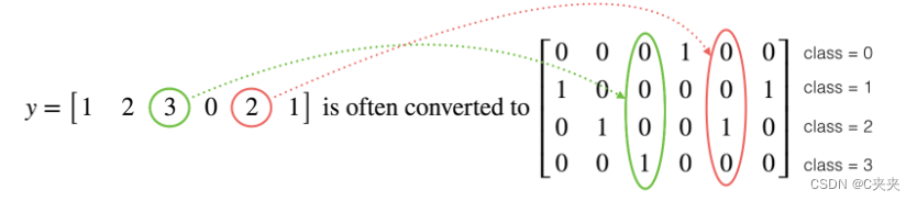
这被称为“一位有效编码”（One Hot Encoding），因为在转换后的表示中，每列恰好有一个元素是“热点”（即设置为1）。在NumPy中，为了进行这种转换，可能需要编写几行代码。而在TensorFlow中，您可以使用一行代码来实现：tf.one_hot(labels, depth, axis)
练习：实现下面的函数，接受一个标签向量和总类别数C，并返回一位有效编码。使用tf.one_hot()来实现。

创建一个矩阵，其中第i行对应于第i个类别编号，第j列对应于第j个训练样本。因此，如果第j个样本具有标签i，则条目(i,j)将为1。
参数：
labels：包含标签的向量
C：类别数量，即一位有效编码维度的深度
返回：
one_hot：一位有效编码矩阵

# GRADED FUNCTION: one_hot_matrix
def one_hot_matrix(labels, C):
    # Create a tf.constant equal to C (depth), name it 'C'. (approx. 1 line)
     C = tf.constant(value = C, name = "C")
    # Use tf.one_hot, be careful with the axis (approx. 1 line)
    one_hot_matrix = tf.one_hot(labels, C, axis = 0)
    # Create the session (approx. 1 line)
    sess = tf.Session()
    # Run the session (approx. 1 line)
    one_hot = sess.run(one_hot_matrix)
    # Close the session (approx. 1 line). See method 1 above.
    sess.close()    
    return one_hot
labels = np.array([1,2,3,0,2,1])
one_hot = one_hot_matrix(labels, C = 4)
print ("one_hot = " + str(one_hot))

在这里插入图片描述

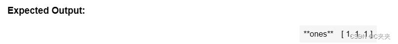
5、使用1和0进行初始化

现在学习如何初始化一个由零和一组成的向量。将调用的函数是tf.ones()。要使用零进行初始化，您可以使用tf.zeros()。这些函数接受一个形状（shape）参数，并返回一个由零或一组成的具有相应维度的数组。
练习：实现下面的函数，接受一个形状参数，并返回一个由一组成的具有相应维度的数组。
tf.ones(shape)

创建一个具有形状为shape的由1组成的数组。
参数：shape：要创建的数组的形状
返回：ones：只包含1的数组

# GRADED FUNCTION: ones
def ones(shape):    
    # Create "ones" tensor using tf.ones(...). (approx. 1 line)
    ones = tf.ones(shape)
    # Create the session (approx. 1 line)
    sess = tf.Session()
    # Run the session to compute 'ones' (approx. 1 line)
    ones = sess.run(ones)
    # Close the session (approx. 1 line). See method 1 above.
    sess.close()
    return ones
print ("ones = " + str(ones([3])))

在这里插入图片描述

二、构建您的第一个TensorFlow神经网络

使用TensorFlow构建一个神经网络模型。
实现TensorFlow模型有两个步骤：
1、创建计算图（Computation Graph）
2、运行计算图

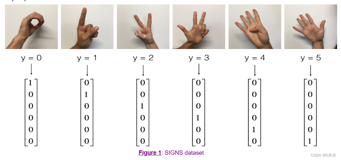
0、问题陈述：SIGNS数据集

构建一个算法，能够帮助语言障碍者与不懂手语的人进行交流。
训练集：1080张表示从0到5的数字的手势的图片（每个数字180张）。
测试集：120张表示从0到5的数字的手势的图片（每个数字20张）。
请注意，这是SIGNS数据集的一个子集。完整的数据集包含更多的手势。
以下是每个数字的示例图片，以及我们如何表示标签的解释。这些是在将图像分辨率降低到64x64像素之前的原始图片。
在这里插入图片描述

# Loading the dataset
X_train_orig, Y_train_orig, X_test_orig, Y_test_orig, classes = load_dataset()
# Example of a picture
index = 70
plt.imshow(X_train_orig[index])
print ("y = " + str(np.squeeze(Y_train_orig[:, index])))

通常情况下，会将图像数据集展平，然后通过除以255进行归一化。此外，您将根据图1所示的方式将每个标签转换为一位有效编码的向量。运行下面的单元格来执行这些操作

# Flatten the training and test images
X_train_flatten = X_train_orig.reshape(X_train_orig.shape[0], -1).T
X_test_flatten = X_test_orig.reshape(X_test_orig.shape[0], -1).T
# Normalize image vectors
X_train = X_train_flatten/255.
X_test = X_test_flatten/255.
# Convert training and test labels to one hot matrices
Y_train = convert_to_one_hot(Y_train_orig, 6)
Y_test = convert_to_one_hot(Y_test_orig, 6)

print ("number of training examples = " + str(X_train.shape[1]))
print ("number of test examples = " + str(X_test.shape[1]))
print ("X_train shape: " + str(X_train.shape))
print ("Y_train shape: " + str(Y_train.shape))
print ("X_test shape: " + str(X_test.shape))
print ("Y_test shape: " + str(Y_test.shape))

请注意，12288来自于64×64×3。每个图像都是64×64像素的正方形，3代表RGB颜色通道。在继续之前，请确保对这些形状有清楚的理解。目标是构建一个能够高精度识别手势的算法。为了实现这个目标，将构建一个几乎与之前在numpy中构建的用于猫识别的模型相同的TensorFlow模型（但现在使用了softmax输出）。这是一个很好的机会，可以将您的numpy实现与TensorFlow实现进行比较。
该模型的结构是：线性层 -> ReLU激活函数 -> 线性层 -> ReLU激活函数 -> 线性层 -> Softmax输出层。这里将SIGMOID输出层转换为了Softmax输出层。Softmax层将SIGMOID推广到多类别分类的情况。

1、创建占位符

第一个任务是创建X和Y的占位符。这将允许在运行会话时传递训练数据。
练习：实现下面的函数，使用TensorFlow创建占位

创建TensorFlow会话的占位符。
参数：
n_x：标量，图像向量的大小（num_px * num_px = 64 * 64 * 3 = 12288）
n_y：标量，类别数量（从0到5，因此 -> 6）
返回：
X：数据输入的占位符，形状为[n_x, None]，数据类型为"float"
Y：输入标签的占位符，形状为[n_y, None]，数据类型为"float"
提示：
使用None是因为它允许我们在占位符的示例数上灵活选择。
实际上，在测试和训练过程中，示例的数量是不同的。

# GRADED FUNCTION: create_placeholders
def create_placeholders(n_x, n_y):
    X = tf.placeholder(tf.float32, shape = [n_x, None])
    Y = tf.placeholder(tf.float32, shape = [n_y, None])
    return X, Y
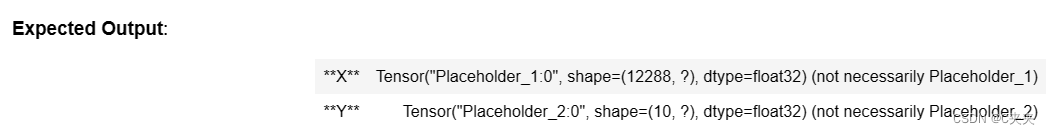
X, Y = create_placeholders(12288, 6)
print ("X = " + str(X))
print ("Y = " + str(Y))

在这里插入图片描述

2、初始化参数

练习：实现下面的函数，使用Xavier初始化权重，并使用零初始化偏置。给出了参数的形状。以下是W1和b1的示例初始化代码：
W1 = tf.get_variable(“W1”, [25,12288], initializer = tf.contrib.layers.xavier_initializer(seed = 1))
b1 = tf.get_variable(“b1”, [25,1], initializer = tf.zeros_initializer())

使用TensorFlow初始化参数来构建神经网络。参数的形状如下：
W1: [25, 12288]
b1: [25, 1]
W2: [12, 25]
b2: [12, 1]
W3: [6, 12]
b3: [6, 1]
返回：parameters：包含W1、b1、W2、b2、W3、b3的张量字典

# GRADED FUNCTION: initialize_parameters
def initialize_parameters():
    tf.set_random_seed(1)                   # so that your "random" numbers match ours
        
    W1 = tf.get_variable("W1", [25,12288], initializer = tf.contrib.layers.xavier_initializer(seed = 1))
    b1 = tf.get_variable("b1", [25,1], initializer = tf.zeros_initializer())
    W2 = tf.get_variable("W2", [12,25], initializer = tf.contrib.layers.xavier_initializer(seed = 1))
    b2 = tf.get_variable("b2", [12,1], initializer = tf.zeros_initializer())
    W3 = tf.get_variable("W3",[6,12], initializer = tf.contrib.layers.xavier_initializer(seed = 1))
    b3 = tf.get_variable("b3", [6,1], initializer = tf.zeros_initializer())

    parameters = {"W1": W1,
                  "b1": b1,
                  "W2": W2,
                  "b2": b2,
                  "W3": W3,
                  "b3": b3}
    
    return parameters
tf.reset_default_graph()
with tf.Session() as sess:
    parameters = initialize_parameters()
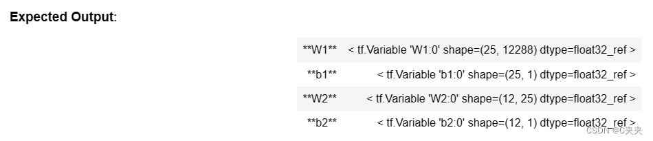
    print("W1 = " + str(parameters["W1"]))
    print("b1 = " + str(parameters["b1"]))
    print("W2 = " + str(parameters["W2"]))
    print("b2 = " + str(parameters["b2"]))

在这里插入图片描述

3、在tensorflow中实现前向传播

该函数将接受一个参数字典，并完成前向传播过程。您将使用以下函数：
tf.add(…, …) 执行加法
tf.matmul(…, …) 执行矩阵乘法
tf.nn.relu(…) 应用ReLU激活函数
问题：实现神经网络的前向传播。已经提供了numpy的等效实现，以便可以将TensorFlow的实现与numpy进行比较。重要的是要注意，在TensorFlow中，前向传播在z3处停止。原因是在TensorFlow中，最后一个线性层的输出将作为输入传递给计算损失的函数。因此，不需要a3！

实现模型的前向传播：线性层 -> ReLU激活函数 -> 线性层 -> ReLU激活函数 -> 线性层 -> Softmax输出层。
参数：
X：输入数据集的占位符，形状为（输入大小，示例数）
parameters：包含参数"W1"、"b1"、"W2"、"b2"、"W3"、"b3"的Python字典，这些参数的形状在初始化参数函数中给出
返回：Z3：最后一个线性单元的输出

# GRADED FUNCTION: forward_propagation
def forward_propagation(X, parameters):
       
    # Retrieve the parameters from the dictionary "parameters" 
    W1 = parameters['W1']
    b1 = parameters['b1']
    W2 = parameters['W2']
    b2 = parameters['b2']
    W3 = parameters['W3']
    b3 = parameters['b3']
    
    # Numpy Equivalents:
    Z1 = tf.add(tf.matmul(W1, X), b1)                      # Z1 = np.dot(W1, X) + b1
    A1 = tf.nn.relu(Z1)                                    # A1 = relu(Z1)
    Z2 = tf.add(tf.matmul(W2, A1), b2)                     # Z2 = np.dot(W2, a1) + b2
    A2 = tf.nn.relu(Z2)                                    # A2 = relu(Z2)
    Z3 = tf.add(tf.matmul(W3, A2), b3)                     # Z3 = np.dot(W3,Z2) + b3    
    return Z3
tf.reset_default_graph()
with tf.Session() as sess:
    X, Y = create_placeholders(12288, 6)
    parameters = initialize_parameters()
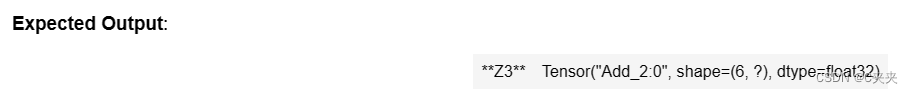
    Z3 = forward_propagation(X, parameters)
    print("Z3 = " + str(Z3))

在这里插入图片描述

4、计算代价

如前所述，使用以下代码非常容易计算成本：tf.reduce_mean(tf.nn.softmax_cross_entropy_with_logits(logits = …, labels = …))
问题：实现下面的成本函数。
需要注意的是，tf.nn.softmax_cross_entropy_with_logits的"logits"和"labels"输入应为形状为（示例数，类别数）的张量。因此，我们已经为您对Z3和Y进行了转置。
此外，tf.reduce_mean基本上对示例进行求和。

计算成本。
参数：
Z3：前向传播的输出（最后一个线性单元的输出），形状为（6，示例数）
Y："真实"标签向量的占位符，与Z3的形状相同
返回：cost：成本函数的张量

# GRADED FUNCTION: compute_cost 
def compute_cost(Z3, Y):
    # to fit the tensorflow requirement for tf.nn.softmax_cross_entropy_with_logits(...,...)
    logits = tf.transpose(Z3)
    labels = tf.transpose(Y)
    
    cost = tf.reduce_mean(tf.nn.softmax_cross_entropy_with_logits(logits = logits, labels = labels))
    return cost
tf.reset_default_graph()
with tf.Session() as sess:
    X, Y = create_placeholders(12288, 6)
    parameters = initialize_parameters()
    Z3 = forward_propagation(X, parameters)
    cost = compute_cost(Z3, Y)
    print("cost = " + str(cost))

5、反向传播和参数更新

所有的反向传播和参数更新都可以在一行代码中完成。将这行代码轻松地整合到模型中非常容易。
在计算成本函数之后，您将创建一个"optimizer"对象。在运行tf.session时，您需要将该对象与成本一起调用。当调用它时，它将使用选择的方法和学习率对给定的成本进行优化。
例如，对于梯度下降，优化器将是：optimizer = tf.train.GradientDescentOptimizer(learning_rate=learning_rate).minimize(cost)
要进行优化，您可以执行以下操作：_, c = sess.run([optimizer, cost], feed_dict={X: minibatch_X, Y: minibatch_Y})
这通过以相反的顺序通过tensorflow图进行反向传播来计算。从成本到输入。
注意：在编码时，我们经常使用_作为一个"丢弃"变量，用于存储我们以后不需要使用的值。在这里，_接收了optimizer的计算值，我们不需要它（而c接收了成本变量的值）。

6、模型建立

实现一个三层的tensorflow神经网络：线性->ReLU->线性->ReLU->线性->Softmax。
参数：
X_train：训练集，形状为（输入大小=12288，训练示例数=1080）
Y_train：训练集标签，形状为（输出大小=6，训练示例数=1080）
X_test：测试集，形状为（输入大小=12288，测试示例数=120）
Y_test：测试集标签，形状为（输出大小=6，测试示例数=120）
learning_rate：优化的学习率
num_epochs：优化循环的迭代次数
minibatch_size：小批量样本的大小
print_cost：是否打印每100个迭代周期的成本
返回：parameters：模型学习到的参数。可以用于预测。

def model(X_train, Y_train, X_test, Y_test, learning_rate = 0.0001,
          num_epochs = 1500, minibatch_size = 32, print_cost = True):   
    
    ops.reset_default_graph()                         # to be able to rerun the model without overwriting tf variables
    tf.set_random_seed(1)                             # to keep consistent results
    seed = 3                                          # to keep consistent results
    (n_x, m) = X_train.shape                          # (n_x: input size, m : number of examples in the train set)
    n_y = Y_train.shape[0]                            # n_y : output size
    costs = []                                        # To keep track of the cost
    
    # Create Placeholders of shape (n_x, n_y)
     X, Y = create_placeholders(n_x, n_y)

    # Initialize parameters
    parameters = initialize_parameters()
    
    # Forward propagation: Build the forward propagation in the tensorflow graph
    Z3 = forward_propagation(X, parameters)
    
    # Cost function: Add cost function to tensorflow graph
    cost = compute_cost(Z3, Y)
    
    # Backpropagation: Define the tensorflow optimizer. Use an AdamOptimizer.
    optimizer = tf.train.AdamOptimizer(learning_rate = learning_rate).minimize(cost)
    
    # Initialize all the variables
    init = tf.global_variables_initializer()

    # Start the session to compute the tensorflow graph
    with tf.Session() as sess:
        
        # Run the initialization
        sess.run(init)
        
        # Do the training loop
        for epoch in range(num_epochs):

            epoch_cost = 0.                       # Defines a cost related to an epoch
            num_minibatches = int(m / minibatch_size) # number of minibatches of size minibatch_size in the train set
            seed = seed + 1
            minibatches = random_mini_batches(X_train, Y_train, minibatch_size, seed)

            for minibatch in minibatches:

                # Select a minibatch
                (minibatch_X, minibatch_Y) = minibatch
                
                # IMPORTANT: The line that runs the graph on a minibatch.
                # Run the session to execute the "optimizer" and the "cost", the feedict should contain a minibatch for (X,Y).
                 _ , minibatch_cost = sess.run([optimizer, cost], feed_dict = {X: minibatch_X, Y: minibatch_Y})
                
                epoch_cost += minibatch_cost / num_minibatches

            # Print the cost every epoch
            if print_cost == True and epoch % 100 == 0:
                print ("Cost after epoch %i: %f" % (epoch, epoch_cost))
            if print_cost == True and epoch % 5 == 0:
                costs.append(epoch_cost)
                
        # plot the cost
        plt.plot(np.squeeze(costs))
        plt.ylabel('cost')
        plt.xlabel('iterations (per tens)')
        plt.title("Learning rate =" + str(learning_rate))
        plt.show()

        # lets save the parameters in a variable
        parameters = sess.run(parameters)
        print ("Parameters have been trained!")

        # Calculate the correct predictions
        correct_prediction = tf.equal(tf.argmax(Z3), tf.argmax(Y))

        # Calculate accuracy on the test set
        accuracy = tf.reduce_mean(tf.cast(correct_prediction, "float"))

        print ("Train Accuracy:", accuracy.eval({X: X_train, Y: Y_train}))
        print ("Test Accuracy:", accuracy.eval({X: X_test, Y: Y_test}))
        
        return parameters
parameters = model(X_train, Y_train, X_test, Y_test)

在这里插入图片描述
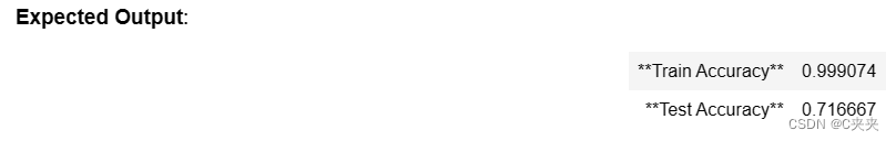
您的算法可以以71.7%的准确率识别表示0到5之间数字的标志。
洞察：您的模型似乎足够大，可以很好地适应训练集。然而，考虑到训练集和测试集准确率之间的差异，您可以尝试添加L2正则化或dropout正则化来减少过拟合。将会话视为训练模型的代码块。每次在小批量上运行会话时，都会训练参数。总共运行了大量次数的会话（1500个迭代周期），直到获得训练良好的参数。

7、用自己的图片进行测试

操作步骤如下：
1、点击笔记本上方的"文件"，然后点击"打开"进入Coursera Hub。
2、将您的图像添加到此Jupyter Notebook的目录中的"images"文件夹中。
3、在下面的代码中写入您的图像名称。
4、运行代码并检查算法是否正确！

import scipy
from PIL import Image
from scipy import ndimage

my_image = "thumbs_up.jpg"

# We preprocess your image to fit your algorithm.
fname = "images/" + my_image
image = np.array(ndimage.imread(fname, flatten=False))
my_image = scipy.misc.imresize(image, size=(64,64)).reshape((1, 64*64*3)).T
my_image_prediction = predict(my_image, parameters)

plt.imshow(image)
print("Your algorithm predicts: y = " + str(np.squeeze(my_image_prediction)))

尽管您可以看到算法似乎将其错误地分类了。原因是训练集中没有包含任何"赞"的样本，所以模型不知道如何处理它！我们称之为"数据分布不匹配"，这是下一个关于"机器学习项目结构化"的课程中的各种问题之一。
记住：
1、Tensorflow是用于深度学习的编程框架。
2、Tensorflow中的两个主要对象类别是Tensors（张量）和Operators（操作符）。
3、在使用tensorflow编码时，您需要执行以下步骤：
1）创建一个包含Tensors（变量、占位符等）和Operations（tf.matmul、tf.add等）的图。
2）创建一个会话（session）。
3）初始化会话。
4）运行会话以执行图。
5）可以像在model()函数中看到的那样多次执行图。
6）当在"optimizer"对象上运行会话时，自动进行反向传播和优化。

C夹夹

关注

0
点赞
踩
0

收藏

觉得还不错? 一键收藏
1
评论
吴恩达深度学习_2_Week3超参数调参、Batch正则化和程序框架(2)

在TensorFlow中完成以下任务：1、初始化变量2、开启自己的会话3、训练算法4、实现神经网络第二门课：改善深层神经网络：超参数调参、正则化以及优化第三周：超参数调参、Batch正则化和程序框架。
复制链接

扫一扫