吴恩达深度学习_4_Week1卷积神经网络(1)

C夹夹

已于 2023-11-13 10:57:20 修改

阅读量80

点赞数

分类专栏：吴恩达深度学习文章标签：深度学习 cnn 人工智能

于 2023-11-12 22:13:57 首次发布

本文链接：https://blog.csdn.net/zxy0000zxy/article/details/134366033

版权

吴恩达深度学习专栏收录该内容

23 篇文章 1 订阅

订阅专栏

卷积神经网络—逐步实现

1、本模型所用函数包
2、任务概述
3、卷积神经网络
4、池化层
5、在池化层中实现后向传播

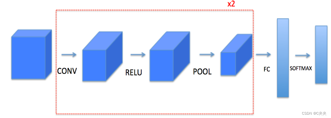
第四门课：卷积神经网络
第一周：卷积神经网络

使用NumPy实现卷积（CONV）和池化（POOL）层，包括正向传播和（可选）反向传播。
符号说明：
上标 [𝑙] 表示第 𝑙 层的对象。
例如：𝑎[4] 是第4层的激活。𝑊[5] 和 𝑏[5] 是第5层的参数。
上标 (𝑖) 表示来自第 𝑖 个示例的对象。
例如：𝑥(𝑖) 是第 𝑖 个训练示例的输入。
下标 𝑖 表示向量的第 𝑖 个条目。
例如：𝑎[𝑙]𝑖 表示第 𝑙 层的激活的第 𝑖 个条目，假设这是一个全连接（FC）层。
𝑛𝐻 ，𝑛𝑊 和 𝑛𝐶 分别表示给定层的高度、宽度和通道数。如果想引用特定的层 𝑙 ，也可以写作 𝑛[𝑙]𝐻 ，𝑛[𝑙]𝑊 ，𝑛[𝑙]𝐶 。
𝑛𝐻𝑝𝑟𝑒𝑣 ，𝑛𝑊𝑝𝑟𝑒𝑣 和 𝑛𝐶𝑝𝑟𝑒𝑣 分别表示前一层的高度、宽度和通道数。如果引用特定的层 𝑙 ，也可以表示为 𝑛[𝑙−1]𝐻 ，𝑛[𝑙−1]𝑊 ，𝑛[𝑙−1]𝐶

一、函数包

import numpy as np
import h5py
import matplotlib.pyplot as plt

plt.rcParams['figure.figsize'] = (5.0, 4.0) # set default size of plots
plt.rcParams['image.interpolation'] = 'nearest'
plt.rcParams['image.cmap'] = 'gray'

np.random.seed(1)

二、任务概述

实现卷积神经网络的构建模块：将实现的每个函数都将有详细的说明，指导完成所需的步骤：
卷积函数，包括：
1、零填充
2、卷积窗口
3、卷积正向传播
4、卷积反向传播
池化函数，包括：
1、池化正向传播
2、创建掩码
3、分发值
4、池化反向传播
使用NumPy从头开始实现这些函数。在下一个节，使用TensorFlow等效的函数来构建以下模型：
在这里插入图片描述
注意：对于每个正向函数，都有相应的反向函数。因此，在正向模块的每个步骤中，将在缓存中存储一些参数。这些参数在反向传播过程中用于计算梯度。

三、卷积神经网络

在这部分中，将构建卷积层的每个步骤。首先，将实现两个辅助函数：一个用于零填充，另一个用于计算卷积函数本身。
在这里插入图片描述

1、零填充

在这里插入图片描述
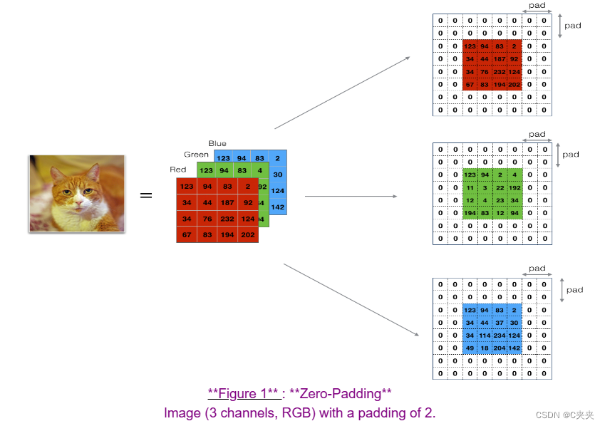
填充的主要好处如下：
1、允许在不必缩小体积的高度和宽度的情况下使用CONV层。这对于构建更深的网络非常重要，否则随着深层的增加，高度/宽度会缩小。一个重要的特例是"same"卷积，在这种情况下，经过一层后高度/宽度完全保持不变。
2、帮助我们保留图像边界的更多信息。如果没有填充，图像边缘的像素对下一层的影响会非常有限。
练习：实现以下函数，用零填充一批示例X的所有图像。使用np.pad函数。注意，如果您想将形状为(5,5,5,5,5)的数组"a"在第2维度上填充1个单位，第4维度上填充3个单位，其他维度上不填充，可以这样做：
a = np.pad(a, ((0,0), (1,1), (0,0), (3,3), (0,0)), ‘constant’, constant_values = (…,…))

使用零填充数据集X中的所有图像。填充应用于图像的高度和宽度。
参数：
  X -- 一个形状为(m, n_H, n_W, n_C)的Python NumPy数组，表示m个图像的批次
  pad -- 整数，每个图像在垂直和水平维度周围的填充量
返回：X_pad -- 填充后的图像，形状为(m, n_H + 2pad, n_W + 2pad, n_C)

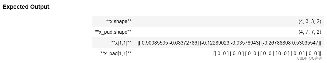
# GRADED FUNCTION: zero_pad
def zero_pad(X, pad):
    X_pad = np.pad(X, ((0,0), (pad,pad), (pad,pad), (0,0)), 'constant')   
     
    return X_pad
    
np.random.seed(1)
x = np.random.randn(4, 3, 3, 2)
x_pad = zero_pad(x, 2)
print ("x.shape =", x.shape)
print ("x_pad.shape =", x_pad.shape)
print ("x[1,1] =", x[1,1])
print ("x_pad[1,1] =", x_pad[1,1])

fig, axarr = plt.subplots(1, 2)
axarr[0].set_title('x')
axarr[0].imshow(x[0,:,:,0])
axarr[1].set_title('x_pad')
axarr[1].imshow(x_pad[0,:,:,0])

在这里插入图片描述

2、卷积的单步操作

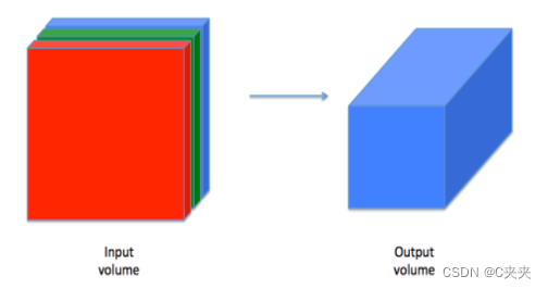
在这部分中，实现卷积的单步操作，其中将过滤器应用于输入的单个位置。这将用于构建卷积单元，其功能如下：
1、接收一个输入体积
2、在输入的每个位置应用过滤器
3、输出另一个体积（通常具有不同的尺寸）
在这里插入图片描述
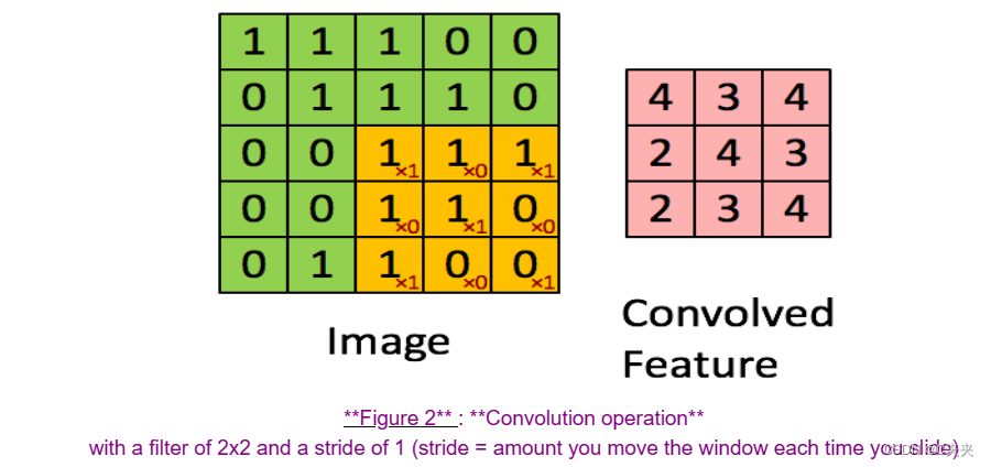
在计算机视觉应用中，左侧矩阵中的每个值对应于单个像素值，通过将3x3过滤器的值与原始矩阵的元素逐个相乘，然后将它们相加并添加偏置来对图像执行卷积。在本练习的第一步中，将实现卷积的单步操作，对应于将过滤器应用于一个位置，以获得单个实值输出。
在本任务的后面部分，将此函数应用于输入的多个位置，以实现完整的卷积操作。
练习：实现conv_single_step()函数。提示：https://docs.scipy.org/doc/numpy-1.13.0/reference/generated/numpy.sum.html

将由参数W定义的一个过滤器应用于前一层输出激活的单个切片(a_slice_prev)。
参数：
a_slice_prev -- 输入数据的切片，形状为(f, f, n_C_prev)
W -- 包含在窗口中的权重参数，形状为(f, f, n_C_prev)
b -- 包含在窗口中的偏置参数，形状为(1, 1, 1)
返回：Z -- 一个标量值，表示在输入数据的切片x上对滑动窗口(W, b)进行卷积的结果

# GRADED FUNCTION: conv_single_step
def conv_single_step(a_slice_prev, W, b):
    # a_slice和W之间的逐元素乘积。尚未添加偏置
    s = a_slice_prev * W
    # 对体积s的所有元素求和
    Z = np.sum(s)
    # 将偏置b添加到Z中。将b转换为float()类型，以便Z结果为标量值。
    Z = Z + b
    return Z
    
np.random.seed(1)
a_slice_prev = np.random.randn(4, 4, 3)
W = np.random.randn(4, 4, 3)
b = np.random.randn(1, 1, 1)

Z = conv_single_step(a_slice_prev, W, b)
print("Z =", Z)

输出结果为：Z -6.99908945068

3、卷积神经网络—前向传播

在这里插入图片描述
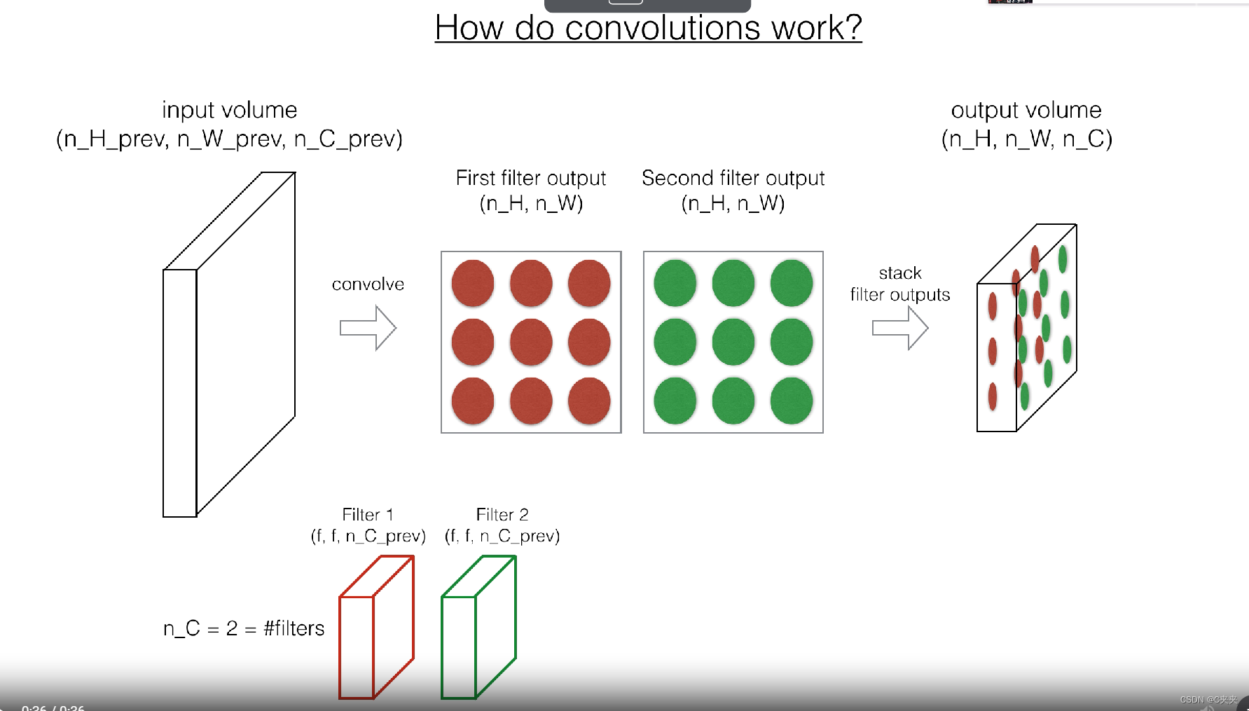
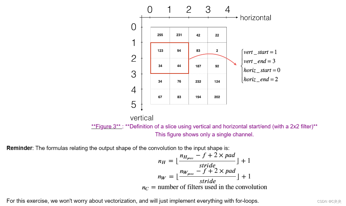
练习：实现以下函数，以在输入激活A_prev上卷积滤波器W。该函数的输入包括A_prev（上一层输出的激活，对于一批m个输入）、用W表示的F个滤波器/权重和用b表示的偏置向量，其中每个滤波器都有自己的（单个）偏置。最后，您还可以访问包含步幅和填充的超参数字典。
提示：
1、要选择矩阵"a_prev"（形状为(5,5,3)）左上角的2x2切片，可以执行以下操作：a_slice_prev = a_prev[0:2,0:2,:]
当定义a_slice_prev时，使用您将定义的起始/结束索引将会很有用。
2、要定义a_slice，您首先需要定义其角点的vert_start、vert_end、horiz_start和horiz_end。下面的图示可能对您有所帮助，以找到如何使用代码中的h、w、f和s来定义每个角点。
在这里插入图片描述

实现卷积函数的前向传播
参数：
A_prev -- 上一层的输出激活，形状为(m, n_H_prev, n_W_prev, n_C_prev)的NumPy数组
W -- 权重，形状为(f, f, n_C_prev, n_C)的NumPy数组
b -- 偏置，形状为(1, 1, 1, n_C)的NumPy数组
hparameters -- 包含"stride"和"pad"的Python字典
返回：
Z -- 卷积输出，形状为(m, n_H, n_W, n_C)的NumPy数组
cache -- conv_backward()函数所需的值的缓存

# GRADED FUNCTION: conv_forward
def conv_forward(A_prev, W, b, hparameters):
    # 1、从A_prev的形状中获取维度
    (m, n_H_prev, n_W_prev, n_C_prev) = A_prev.shape
    
    # 2、从W的形状中获取维度
    (f, f, n_C_prev, n_C) = W.shape
    
    # 3、从"hparameters"中获取信息
    stride = hparameters["stride"]
    pad = hparameters["pad"]

     # 4、使用上述给定的公式计算CONV输出体积的维度。提示：使用int()向下取整
    n_H = int((n_H_prev - f + 2*pad) / stride + 1)
    n_W = int((n_W_prev - f + 2*pad) / stride + 1)

    # 5、用零初始化输出体积Z
    Z = np.zeros((m, n_H, n_W, n_C))
    
    # 6、通过对A_prev进行填充，创建A_prev_pad
    A_prev_pad = zero_pad(A_prev, pad)

    for i in range(m):                                 # loop over the batch of training examples
        a_prev_pad = A_prev_pad[i, :, :, :]            # Select ith training example's padded activation
        for h in range(n_H):                           # loop over vertical axis of the output volume
            for w in range(n_W):                       # loop over horizontal axis of the output volume
                for c in range(n_C):                   # loop over channels (= #filters) of the output volume
           
                    # 7、找到当前“slice”的角点
                    vert_start = stride * h
                    vert_end = vert_start + f
                    horiz_start = stride * w
                    horiz_end = horiz_start + f
            
                    # 8、使用角点定义a_prev_pad的（3D）切片（参见上方的提示） 
                    a_slice_prev = a_prev_pad[vert_start:vert_end, horiz_start:horiz_end, :]

        
                    # 9、将（3D）切片与正确的过滤器W和偏置b进行卷积，以得到一个输出神经元
                    Z[i, h, w, c] = conv_single_step(a_slice_prev, W[:, :, :, c], b[:, :, :, c])
    
    # 10、Making sure your output shape is correct
    assert(Z.shape == (m, n_H, n_W, n_C))
    
    # 11、Save information in "cache" for the backprop
    cache = (A_prev, W, b, hparameters)
    
    return Z, cache
    
np.random.seed(1)
A_prev = np.random.randn(10,4,4,3)
W = np.random.randn(2,2,3,8)
b = np.random.randn(1,1,1,8)
hparameters = {"pad" : 2,"stride": 2}

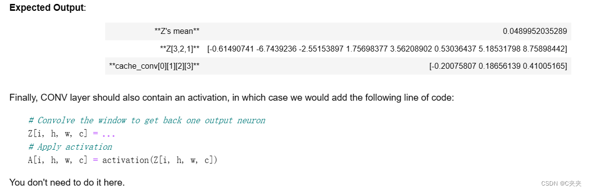
Z, cache_conv = conv_forward(A_prev, W, b, hparameters)
print("Z's mean =", np.mean(Z))
print("Z[3,2,1] =", Z[3,2,1])
print("cache_conv[0][1][2][3] =", cache_conv[0][1][2][3])

在这里插入图片描述

4、池化层

池化（POOL）层减小了输入的高度和宽度。它有助于减少计算量，并使特征检测器对输入中的位置更加不变。池化层有两种类型：
1、最大池化层：在输入上滑动一个（f, f）窗口，并将窗口中的最大值存储在输出中。
2、平均池化层：在输入上滑动一个（f, f）窗口，并将窗口中的平均值存储在输出中。
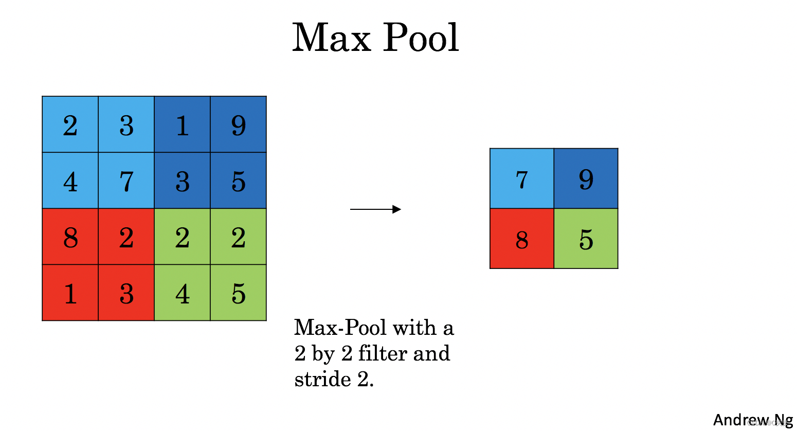在这里插入图片描述这些池化层没有用于反向传播训练的参数。然而，它们有超参数，例如窗口大小f。这指定了计算最大值或平均值的fxf窗口的高度和宽度。

1、前向池化

现在，将在同一个函数中实现MAX-POOL和AVG-POOL。
练习：实现池化层的前向传播。请按照下面注释中的提示进行操作。
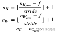
提醒：由于没有填充，将池化层的输出形状与输入形状绑定的公式如下：
在这里插入图片描述

实现池化层的前向传播
参数：
A_prev -- 输入数据，形状为(m, n_H_prev, n_W_prev, n_C_prev)的NumPy数组
hparameters -- 包含"f"和"stride"的Python字典
mode -- 您想要使用的池化模式，定义为字符串（"max"或"average"）
返回：
A -- 池化层的输出，形状为(m, n_H, n_W, n_C)的NumPy数组
cache -- 在池化层的反向传播中使用的缓存，包含输入和hparameters

# GRADED FUNCTION: pool_forward
def pool_forward(A_prev, hparameters, mode = "max"):
 
    # Retrieve dimensions from the input shape
    (m, n_H_prev, n_W_prev, n_C_prev) = A_prev.shape
    # Retrieve hyperparameters from "hparameters"
    f = hparameters["f"]
    stride = hparameters["stride"]
    # Define the dimensions of the output
    n_H = int(1 + (n_H_prev - f) / stride)
    n_W = int(1 + (n_W_prev - f) / stride)
    n_C = n_C_prev
    # Initialize output matrix A
    A = np.zeros((m, n_H, n_W, n_C))              
    
    for i in range(m):                          # loop over the training examples
        for h in range(n_H):                     # loop on the vertical axis of the output volume
            for w in range(n_W):                 # loop on the horizontal axis of the output volume
                for c in range (n_C):            # loop over the channels of the output volume
                    
                    # Find the corners of the current "slice" (≈4 lines) 
                    vert_start = h * stride
                    vert_end = vert_start + f
                    horiz_start = w * stride
                    horiz_end = horiz_start + f
 
                    # Use the corners to define the current slice on the ith training example of A_prev, channel c. 
                     a_prev_slice = A_prev[i, vert_start:vert_end, horiz_start:horiz_end, c]
                    # 对切片执行池化操作。使用if语句区分不同的模式。使用np.max/np.mean函数。
                    if mode == "max":
                        A[i, h, w, c] = np.max(a_prev_slice)
                    elif mode == "average":
                        A[i, h, w, c] = np.mean(a_prev_slice)
   
    # Store the input and hparameters in "cache" for pool_backward()
    cache = (A_prev, hparameters)
    # Making sure your output shape is correct
    assert(A.shape == (m, n_H, n_W, n_C))
    
    return A, cache
    
np.random.seed(1)
A_prev = np.random.randn(2, 4, 4, 3)
hparameters = {"stride" : 2, "f": 3}

A, cache = pool_forward(A_prev, hparameters)
print("mode = max")
print("A =", A)
print()
A, cache = pool_forward(A_prev, hparameters, mode = "average")
print("mode = average")
print("A =", A)

在这里插入图片描述

五、在卷积神经网络中实现后向传播

在现代深度学习框架中，只需要实现前向传播，框架会处理反向传播，因此大多数深度学习工程师不需要关心反向传播的细节。卷积网络的反向传播比较复杂。然而，如果您愿意，可以通过完成本笔记本的可选部分来了解卷积网络中反向传播的工作原理。
在早期的课程中，您实现了一个简单的（全连接）神经网络时，使用反向传播计算了相对于成本的导数以更新参数。类似地，在卷积神经网络中，可以计算相对于成本的导数以更新参数。反向传播方程不是微不足道的，我们在讲座中没有推导出它们，但我们在下面简要地介绍了它们。

1、卷积层的反向传播

从实现CONV层的反向传播开始：
1、计算 dA：
这是计算特定滤波器 Wc 和给定训练示例的成本导数 dA 的公式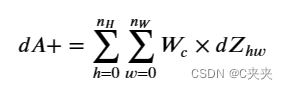：在这里插入图片描述
其中 Wc 是一个滤波器，dZhw 是与 conv 层输出 Z 的第 h 行和第 w 列（对应于第 i 个 stride 向左和第 j 个 stride 向下取的点积）的成本梯度对应的标量。请注意，每次更新 dA 时，我们将相同的滤波器 Wc 乘以不同的 dZ。我们之所以这样做，主要是因为在计算前向传播时，每个滤波器都是由不同的 a_slice 进行点积和求和的。因此，在计算 dA 的反向传播时，我们只是将所有 a_slice 的梯度相加。
在代码中，在适当的 for 循环内，此公式转化为：
da_prev_pad[vert_start:vert_end, horiz_start:horiz_end, :] += W[:,:,:,c] * dZ[i, h, w, c]
2、计算 dW：
这是计算一个滤波器的导数 dWc（dWc 是一个滤波器的导数）相对于损失的公式：
在这里插入图片描述
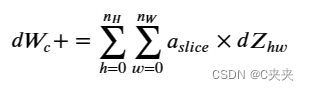
其中 aslice 对应于用于生成 acitivation Zij 的切片。因此，这最终给出了相对于该切片的 W 的梯度。由于是相同的 W，我们将所有这些梯度相加以得到 dW。
在代码中，在适当的 for 循环内，此公式转化为：
dW[:,:,:,c] += a_slice * dZ[i, h, w, c]
3、计算 db：
这是计算特定滤波器 Wc 的成本导数 db 的公式：
db = ∑h ∑w dZhw (3)
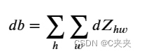
如之前在基本神经网络中看到的那样，db 是通过对 dZ 求和来计算的。在这种情况下，您只是对 conv 输出 Z 相对于成本的所有梯度进行求和。
在代码中，在适当的 for 循环内，此公式转化为：
db[:,:,:,c] += dZ[i, h, w, c]
练习：实现以下 conv_backward 函数。您应该对所有的训练示例、滤波器、高度和宽度进行求和。然后，使用上述公式 1、2 和 3 计算导数。

实现卷积函数的反向传播
参数：
dZ -- 相对于卷积层输出(Z)的成本梯度，形状为(m, n_H, n_W, n_C)的numpy数组
cache -- 用于conv_backward()的值缓存，conv_forward()的输出
返回：
dA_prev -- 相对于卷积层输入(A_prev)的成本梯度，形状为(m, n_H_prev, n_W_prev, n_C_prev)的numpy数组
dW -- 相对于卷积层权重(W)的成本梯度，形状为(f, f, n_C_prev, n_C)的numpy数组
db -- 相对于卷积层偏置(b)的成本梯度，形状为(1, 1, 1, n_C)的numpy数组

def conv_backward(dZ, cache):
    # Retrieve information from "cache"
    (A_prev, W, b, hparameters) = cache

    # Retrieve dimensions from A_prev's shape
    (m, n_H_prev, n_W_prev, n_C_prev) = A_prev.shape

    # Retrieve dimensions from W's shape
    (f, f, n_C_prev, n_C) = W.shape
    
    # Retrieve information from "hparameters"
    stride = hparameters['stride']
    pad = hparameters['pad']

    # Retrieve dimensions from dZ's shape
     (m, n_H, n_W, n_C) = dZ.shape

    # Initialize dA_prev, dW, db with the correct shapes
    dA_prev = np.zeros((m, n_H_prev, n_W_prev, n_C_prev))
    dW = np.zeros((f, f, n_C_prev, n_C))
    db = np.zeros((1, 1, 1, n_C))

    # Pad A_prev and dA_prev
    A_prev_pad = zero_pad(A_prev, pad)
    dA_prev_pad = zero_pad(dA_prev, pad)

    for i in range(m):                       # loop over the training examples

        # select ith training example from A_prev_pad and dA_prev_pad
        a_prev_pad = A_prev_pad[i, :, :, :]
        da_prev_pad = dA_prev_pad[i, :, :, :]

        for h in range(n_H):                   # loop over vertical axis of the output volume
            for w in range(n_W):               # loop over horizontal axis of the output volume
                for c in range(n_C):           # loop over the channels of the output volume

                    # Find the corners of the current "slice"
                    vert_start = h * stride
                    vert_end = vert_start + f
                    horiz_start = w * stride
                    horiz_end = horiz_start + f

                    # Use the corners to define the slice from a_prev_pad
                    a_slice = a_prev_pad[vert_start:vert_end, horiz_start:horiz_end, :]
                    
                    # Update gradients for the window and the filter's parameters using the code formulas given above
                    da_prev_pad[vert_start:vert_end, horiz_start:horiz_end, :] += W[:,:,:,c] * dZ[i, h, w, c]
                    dW[:,:,:,c] += a_slice * dZ[i, h, w, c]
                    db[:,:,:,c] += dZ[i, h, w, c]
             
        # Set the ith training example's dA_prev to the unpaded da_prev_pad (Hint: use X[pad:-pad, pad:-pad, :])
        dA_prev[i, :, :, :] = da_prev_pad[pad:-pad, pad:-pad, :]
    
    # Making sure your output shape is correct
    assert(dA_prev.shape == (m, n_H_prev, n_W_prev, n_C_prev))
    
    return dA_prev, dW, db
    
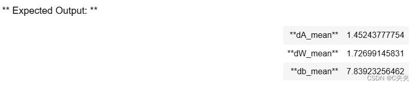
np.random.seed(1)
dA, dW, db = conv_backward(Z, cache_conv)
print("dA_mean =", np.mean(dA))
print("dW_mean =", np.mean(dW))
print("db_mean =", np.mean(db))

在这里插入图片描述

2、池化层反向传播

接下来，让我们来实现池化层的反向传播，首先是MAX-POOL层。尽管池化层没有需要更新的反向传播参数，但你仍然需要通过池化层进行反向传播，以计算出在池化层之前的层的梯度。
1、最大池化 - 反向传播
在开始池化层的反向传播之前，你将构建一个名为create_mask_from_window()的辅助函数，该函数执行以下操作：
在这里插入图片描述
如你所见，此函数创建了一个“掩码”矩阵，用于跟踪矩阵中的最大值位置。True (1) 表示 X 中的最大值位置，其他条目为 False (0)。稍后你将看到，平均池化的反向传播将类似，但使用不同的掩码。
练习：实现 create_mask_from_window()。这个函数对于池化的反向传播将会很有帮助。提示：
1、np.max() 可能会有帮助。它可以计算数组的最大值。
2、如果你有一个矩阵 X 和一个标量 x：A = (X == x) 将返回一个与 X 大小相同的矩阵 A，使得：
A[i,j] = True，如果 X[i,j] = x
A[i,j] = False，如果 X[i,j] != x
3、在这里，你不需要考虑矩阵中存在多个最大值的情况。

从输入矩阵x创建一个掩码，用于标识x的最大条目。
参数：x -- 形状为(f, f)的数组
返回：mask -- 与窗口大小相同的数组，其中在与x的最大条目对应的位置处包含True。

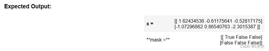
def create_mask_from_window(x):
    mask = (x == np.max(x))
    
    return mask
     
np.random.seed(1)
x = np.random.randn(2,3)
mask = create_mask_from_window(x)
print('x = ', x)
print("mask = ", mask)

在这里插入图片描述
为什么我们要跟踪最大值的位置呢？因为这是最终影响输出和成本的输入值，所以反向传播计算的是相对于成本的梯度，因此任何影响最终成本的因素都应该具有非零梯度。因此，反向传播将梯度"传播"回影响成本的特定输入值。
2、平均池化 - 反向传播
在最大池化中，对于每个输入窗口，输出的所有"影响"都来自一个单独的输入值–最大值。在平均池化中，输入窗口的每个元素对输出具有相等的影响。因此，为了实现反向传播，你现在将实现一个反映这一点的辅助函数。
例如，如果我们在前向传播中使用2x2过滤器进行平均池化，那么在反向传播中使用的掩码将如下所示：
在这里插入图片描述
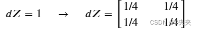
这意味着矩阵𝑑𝑍中的每个位置对输出的贡献是相等的，因为在前向传播中，我们取了平均值。
练习：实现下面的函数，将一个值dz均匀分布到形状为shape的矩阵中。提示：https://docs.scipy.org/doc/numpy-1.13.0/reference/generated/numpy.ones.html

 Distributes the input value in the matrix of dimension shape  
    Arguments:
    dz -- input scalar
    shape -- the shape (n_H, n_W) of the output matrix for which we want to distribute the value of dz 
    Returns:
    a -- Array of size (n_H, n_W) for which we distributed the value of dz

def distribute_value(dz, shape):

    # Retrieve dimensions from shape (≈1 line)
    (n_H, n_W) = shape
  
    # Compute the value to distribute on the matrix (≈1 line)
    average = dz / (n_H * n_W)

    # Create a matrix where every entry is the "average" value (≈1 line)
    a = average * np.ones(shape)
    return a
 a = distribute_value(2, (2,2))
print('distributed value =', a)

distributed_value = [[ 0.5 0.5] [ 0.5 0.5]]
3、融合一起
现在你拥有计算池化层反向传播所需的一切。
练习：在两种模式(“max"和"average”)下实现pool_backward函数。你将再次使用4个for循环(遍历训练样本、高度、宽度和通道)。你应该使用if/elif语句来判断模式是否等于’max’或’average’。如果等于’average’，你应该使用上面实现的distribute_value()函数来创建与a_slice形状相同的矩阵。否则，模式等于’max’，你将使用create_mask_from_window()创建一个掩码，并将其与dZ的相应值相乘。

实现池化层的反向传播。
参数：
dA：关于池化层输出的成本梯度，与A具有相同的形状。
cache：从池化层前向传播的缓存输出，包含该层的输入和超参数。
mode：希望使用的池化模式，定义为字符串("max"或"average")。
返回：
dA_prev：关于池化层输入的成本梯度，与A_prev具有相同的形状。

def pool_backward(dA, cache, mode = "max"):
    # Retrieve information from cache (≈1 line)
    (A_prev, hparameters) = cache

    # Retrieve hyperparameters from "hparameters" (≈2 lines)
    stride = hparameters['stride']
    f = hparameters['f']

    # Retrieve dimensions from A_prev's shape and dA's shape (≈2 lines)
    m, n_H_prev, n_W_prev, n_C_prev = A_prev.shape
    m, n_H, n_W, n_C = dA.shape
 
    # Initialize dA_prev with zeros (≈1 line)
    dA_prev = np.zeros(np.shape(A_prev))
    
    for i in range(m):                       # loop over the training examples

        # select training example from A_prev (≈1 line)
        a_prev = A_prev[i, :, :, :]

        for h in range(n_H):                   # loop on the vertical axis
            for w in range(n_W):               # loop on the horizontal axis
                for c in range(n_C):           # loop over the channels (depth)
        
                    # Find the corners of the current "slice" (≈4 lines)
                    
                    vert_start = h * stride
                    vert_end = vert_start + f
                    horiz_start = w * stride
                    horiz_end = horiz_start + f

                    # Compute the backward propagation in both modes.
                    if mode == "max":
      
                        # Use the corners and "c" to define the current slice from a_prev (≈1 line)
                        a_prev_slice = a_prev[vert_start:vert_end, horiz_start:horiz_end, c]
        

                        # Create the mask from a_prev_slice (≈1 line)
                        mask = create_mask_from_window(a_prev_slice)

                        # Set dA_prev to be dA_prev + (the mask multiplied by the correct entry of dA) (≈1 line)
                        dA_prev[i, vert_start: vert_end, horiz_start: horiz_end, c] += np.multiply(mask, dA[i, h, w, c])
                   
                elif mode == "average":
   
                        # Get the value a from dA (≈1 line)
                        da = dA[i, h, w, c]

                        # Define the shape of the filter as fxf (≈1 line)
                        shape = (f, f)

                        # Distribute it to get the correct slice of dA_prev. i.e. Add the distributed value of da. (≈1 line)
                         dA_prev[i, vert_start: vert_end, horiz_start: horiz_end, c] += distribute_value(da, shape)


    # Making sure your output shape is correct
    assert(dA_prev.shape == A_prev.shape)
    
    return dA_prev
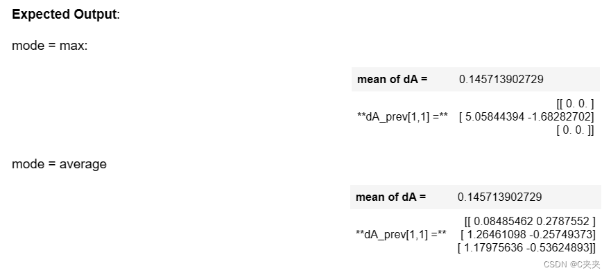
np.random.seed(1)
A_prev = np.random.randn(5, 5, 3, 2)
hparameters = {"stride" : 1, "f": 2}
A, cache = pool_forward(A_prev, hparameters)
dA = np.random.randn(5, 4, 2, 2)

dA_prev = pool_backward(dA, cache, mode = "max")
print("mode = max")
print('mean of dA = ', np.mean(dA))
print('dA_prev[1,1] = ', dA_prev[1,1])  
print()
dA_prev = pool_backward(dA, cache, mode = "average")
print("mode = average")
print('mean of dA = ', np.mean(dA))
print('dA_prev[1,1] = ', dA_prev[1,1])

在这里插入图片描述

C夹夹

关注

0
点赞
踩
0

收藏

觉得还不错? 一键收藏
1
评论
吴恩达深度学习_4_Week1卷积神经网络(1)

实现卷积神经网络的构建模块：将实现的每个函数都将有详细的说明，指导完成所需的步骤：卷积函数，包括：1、零填充2、卷积窗口3、卷积正向传播4、卷积反向传播池化函数，包括：1、池化正向传播2、创建掩码3、分发值4、池化反向传播使用NumPy从头开始实现这些函数。在下一个节，使用TensorFlow等效的函数来构建以下模型：注意：对于每个正向函数，都有相应的反向函数。因此，在正向模块的每个步骤中，将在缓存中存储一些参数。这些参数在反向传播过程中用于计算梯度。
复制链接

扫一扫