


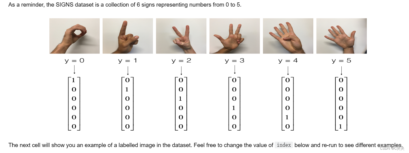
卷积神经网络—应用
1、TensorFlow模型
2、创建占位符
3、初始化参数
4、前向传播
5、计算代价
6、模型
第四门课:卷积神经网络
第一周:卷积神经网络
本Task:
1、实现在实现TensorFlow模型时会用到的辅助函数
2、使用TensorFlow实现一个完整的ConvNet
完成这个后,将能够:在TensorFlow中构建和训练一个用于分类问题的ConvNet
一、TensorFlow模型
大多数实际应用的深度学习都使用编程框架构建,这些框架中有许多内置的函数可以直接调用
import math
import numpy as np
import h5py
import matplotlib.pyplot as plt
import scipy
from PIL import Image
from scipy import ndimage
import tensorflow as tf
from tensorflow.python.framework import ops
from cnn_utils import *

np.random.seed(1)

# Loading the data (signs)
X_train_orig, Y_train_orig, X_test_orig, Y_test_orig, classes = load_dataset()
# Example of a picture
index = 15
plt.imshow(X_train_orig[index])
print ("y = " + str(np.squeeze(Y_train_orig[:, index])))
测试数据的维度
X_train = X_train_orig/255.
X_test = X_test_orig/255.
Y_train = convert_to_one_hot(Y_train_orig, 6).T
Y_test = convert_to_one_hot(Y_test_orig, 6).T
print ("number of training examples = " + str(X_train.shape[0]))
print ("number of test examples = " + str(X_test.shape[0]))
print ("X_train shape: " + str(X_train.shape))
print ("Y_train shape: " + str(Y_train.shape))
print ("X_test shape: " + str(X_test.shape))
print ("Y_test shape: " + str(Y_test.shape))
conv_layers = {}
二、创建占位符
在TensorFlow中,当运行会话时,需要为输入数据创建占位符。
练习:实现下面的函数,为输入图像X和输出Y创建占位符。你现在不需要定义训练样本的数量。你可以使用"None"作为批量大小,这样可以在稍后选择。因此,X应该具有维度[None,n_H0,n_W0,n_C0],Y应该具有维度[None,n_y]。提示
创建TensorFlow会话的占位符。
参数:
n_H0:标量,输入图像的高度
n_W0:标量,输入图像的宽度
n_C0:标量,输入的通道数
n_y:标量,类别的数量
返回:
X:数据输入的占位符,形状为[None, n_H0, n_W0, n_C0],数据类型为"float"
Y:输入标签的占位符,形状为[None, n_y],数据类型为"float"
# GRADED FUNCTION: create_placeholders
def create_placeholders(n_H0, n_W0, n_C0, n_y):
X = tf.placeholder(tf.float32, shape=[None, n_H0, n_W0, n_C0])
Y = tf.placeholder(tf.float32, shape=[None, n_y])
return X, Y
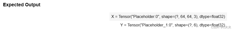
X, Y = create_placeholders(64, 64, 3, 6)
print ("X = " + str(X))
print ("Y = " + str(Y))
三、初始化参数
将使用tf.contrib.layers.xavier_initializer(seed = 0)初始化权重/滤波器𝑊1和𝑊2。不需要担心偏差变量,因为很快会看到TensorFlow的函数会处理偏差。注意,只需要初始化conv2d函数中的权重/滤波器。TensorFlow会自动初始化全连接部分的层。
练习:实现initialize_parameters()函数。下面提供了每组滤波器的维度。提醒一下,在Tensorflow中,要初始化形状为[1,2,3,4]的参数𝑊,可以使用以下方式:W = tf.get_variable(“W”, [1,2,3,4], initializer = …)
more info
使用TensorFlow初始化权重参数来构建神经网络。形状如下:
W1:[4, 4, 3, 8]
W2:[2, 2, 8, 16]
返回:parameters -- 包含W1,W2的张量字典
# GRADED FUNCTION: initialize_parameters
def initialize_parameters():
tf.set_random_seed(1) # so that your "random" numbers match ours
W1 = tf.get_variable("W1", [4, 4, 3, 8], initializer=tf.contrib.layers.xavier_initializer(seed=0))
W2 = tf.get_variable("W2", [2, 2, 8, 16], initializer=tf.contrib.layers.xavier_initializer(seed=0))
parameters = {"W1": W1,
"W2": W2}
return parameters
tf.reset_default_graph()
with tf.Session() as sess_test:
parameters = initialize_parameters()
init = tf.global_variables_initializer()
sess_test.run(init)
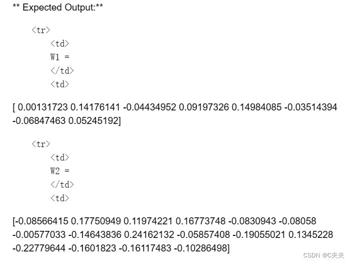
print("W1 = " + str(parameters["W1"].eval()[1,1,1]))
print("W2 = " + str(parameters["W2"].eval()[1,1,1]))
四、前向传播
在TensorFlow中,有一些内置函数可以执行卷积步骤。
1、tf.nn.conv2d(X, W1, strides=[1,s,s,1], padding=‘SAME’):给定输入𝑋和一组滤波器𝑊1,该函数在𝑋上进行𝑊1的卷积操作。第三个输入参数([1,f,f,1])表示输入的每个维度(m, n_H_prev, n_W_prev, n_C_prev)的步长。你可以在这里阅读完整的文档
2、tf.nn.max_pool(A, ksize=[1,f,f,1], strides=[1,s,s,1], padding=‘SAME’):给定输入A,该函数使用大小为(f, f)和步长为(s, s)的窗口在每个窗口上进行最大池化。阅读完整文档
3、tf.nn.relu(Z1):计算Z1的逐元素ReLU(可以是任意形状。阅读完整文档
4、tf.contrib.layers.flatten§:给定输入P,该函数将每个样本展平为一个1D向量,同时保持批量大小。它返回一个形状为[batch_size, k]的展平张量。阅读完整文档
5、tf.contrib.layers.fully_connected(F, num_outputs):给定展平输入F,它使用全连接层计算输出。阅读完整文档
在上面的最后一个函数(tf.contrib.layers.fully_connected)中,全连接层会在图中自动初始化权重,并在训练模型时不断进行训练。因此,在初始化参数时不需要初始化这些权重。
练习:
实现下面的forward_propagation函数来构建以下模型:CONV2D -> RELU -> MAXPOOL -> CONV2D -> RELU -> MAXPOOL -> FLATTEN -> FULLYCONNECTED。你应该使用上面提到的函数。
具体而言,我们将对所有步骤使用以下参数:
Conv2D:步长为1,填充为"SAME"
ReLU
Max pool:使用8x8的过滤器大小和8x8的步长,填充为"SAME"
Conv2D:步长为1,填充为"SAME"
ReLU
Max pool:使用4x4的过滤器大小和4x4的步长,填充为"SAME"
将前面的输出展平
FULLYCONNECTED(FC)层:应用一个没有非线性激活函数的全连接层。这里不要调用softmax。这将导致输出层中有6个神经元,然后稍后将它们传递给softmax。在TensorFlow中,softmax和损失函数被组合成一个单独的函数,你将在计算损失时调用该函数。
为模型实现前向传播:
CONV2D -> RELU -> MAXPOOL -> CONV2D -> RELU -> MAXPOOL -> FLATTEN -> FULLYCONNECTED
参数:
X -- 输入数据集的占位符,形状为(输入大小,样本数)
parameters -- 包含参数"W1"、"W2"的Python字典,这些参数的形状在initialize_parameters函数中给出
返回:Z3 -- 最后一个线性单元的输出
# GRADED FUNCTION: forward_propagation
def forward_propagation(X, parameters):
# Retrieve the parameters from the dictionary "parameters"
W1 = parameters['W1']
W2 = parameters['W2']
# CONV2D: stride of 1, padding 'SAME'
Z1 = tf.nn.conv2d(X, W1, strides=[1,1,1,1], padding='SAME')
# RELU
A1 = tf.nn.relu(Z1)
# MAXPOOL: window 8x8, sride 8, padding 'SAME'
P1 = tf.nn.max_pool(A1, ksize=[1,8,8,1], strides=[1,8,8,1], padding='SAME')
# CONV2D: filters W2, stride 1, padding 'SAME'
Z2 = tf.nn.conv2d(P1, W2, strides=[1,1,1,1], padding='SAME')
# RELU
A2 = tf.nn.relu(Z2)
# MAXPOOL: window 4x4, stride 4, padding 'SAME'
P2 = tf.nn.max_pool(A2, ksize=[1,4,4,1], strides=[1,4,4,1], padding='SAME')
# FLATTEN
P2 = tf.contrib.layers.flatten(P2)
# FULLY-CONNECTED without non-linear activation function (not not call softmax).
# 6 neurons in output layer. Hint: one of the arguments should be "activation_fn=None"
Z3 = tf.contrib.layers.fully_connected(P2, 6, activation_fn=None)
return Z3
tf.reset_default_graph()
with tf.Session() as sess:
np.random.seed(1)
X, Y = create_placeholders(64, 64, 3, 6)
parameters = initialize_parameters()
Z3 = forward_propagation(X, parameters)
init = tf.global_variables_initializer()
sess.run(init)
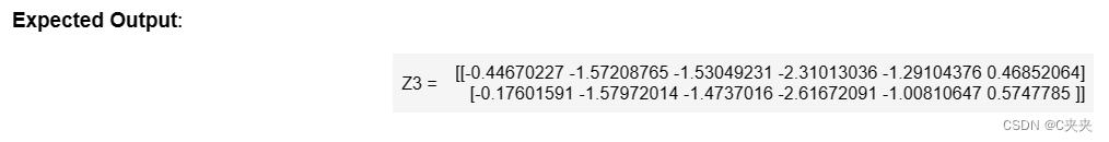
a = sess.run(Z3, {X: np.random.randn(2,64,64,3), Y: np.random.randn(2,6)})
print("Z3 = " + str(a))
五、计算代价
实现下面的计算损失函数。你可能会发现以下两个函数很有帮助:
1、tf.nn.softmax_cross_entropy_with_logits(logits=Z3, labels=Y):计算softmax交叉熵损失。该函数既计算softmax激活函数,也计算结果损失。完整文档
2、tf.reduce_mean:计算张量在各个维度上的元素的均值。使用它将所有示例上的损失求和以获得总体成本。完整文档
练习:使用上面的函数计算下面的成本。
计算成本
参数:
Z3 -- 前向传播的输出(最后一个线性单元的输出),形状为(6,样本数)
Y -- "true"标签向量的占位符,与Z3形状相同
返回:cost - 成本函数的张量
# GRADED FUNCTION: compute_cost
def compute_cost(Z3, Y):
    cost = tf.reduce_mean(tf.nn.softmax_cross_entropy_with_logits(logits = Z3, labels = Y))

    return cost
tf.reset_default_graph()
with tf.Session() as sess:
    np.random.seed(1)
    X, Y = create_placeholders(64, 64, 3, 6)
    parameters = initialize_parameters()
    Z3 = forward_propagation(X, parameters)
    cost = compute_cost(Z3, Y)
    init = tf.global_variables_initializer()
    sess.run(init)
    a = sess.run(cost, {X: np.random.randn(4,64,64,3), Y: np.random.randn(4,6)})
    print("cost = " + str(a))
cost=2.91034
六、模型
最后,你将合并上面实现的辅助函数来构建一个模型,并在SIGNS数据集上进行训练。
已经实现了random_mini_batches()。请记住,该函数返回一个迷你批次的列表。
练习:完成下面的函数。下面的模型应该:
1、创建占位符
2、初始化参数
3、进行前向传播
4、计算成本
5、创建一个优化器
最后,你将创建一个会话,并运行一个循环进行num_epochs次训练,获取迷你批次,然后对每个迷你批次进行优化。关于变量初始化的提示
在TensorFlow中实现一个三层的卷积神经网络:
CONV2D -> RELU -> MAXPOOL -> CONV2D -> RELU -> MAXPOOL -> FLATTEN -> FULLYCONNECTED
参数:
X_train -- 训练集,形状为(None,64,64,3)
Y_train -- 测试集,形状为(None,n_y = 6)
X_test -- 训练集,形状为(None,64,64,3)
Y_test -- 测试集,形状为(None,n_y = 6)
learning_rate -- 优化的学习率
num_epochs -- 优化循环的迭代次数
minibatch_size -- 迷你批次的大小
print_cost -- 是否打印每100个迭代周期的成本
返回:
train_accuracy -- 实数,训练集(X_train)上的准确率
test_accuracy -- 实数,测试集(X_test)上的准确率
parameters -- 模型学习到的参数。然后可以用于预测。
# GRADED FUNCTION: model
def model(X_train, Y_train, X_test, Y_test, learning_rate = 0.009,
          num_epochs = 100, minibatch_size = 64, print_cost = True):

    ops.reset_default_graph()                         # 为了能够重新运行模型而不覆盖 TensorFlow 变量
    tf.set_random_seed(1)                             # to keep results consistent (tensorflow seed)
    seed = 3                                          # to keep results consistent (numpy seed)
    (m, n_H0, n_W0, n_C0) = X_train.shape
    n_y = Y_train.shape[1]
    costs = []                                        # To keep track of the cost

    # Create Placeholders of the correct shape
    X, Y = create_placeholders(n_H0, n_W0, n_C0, n_y)
    # Initialize parameters
    parameters = initialize_parameters()
    # Forward propagation: Build the forward propagation in the tensorflow graph
    Z3 = forward_propagation(X, parameters)
    # Cost function: Add cost function to tensorflow graph
    cost = compute_cost(Z3, Y)
    # Backpropagation: Define the tensorflow optimizer. Use an AdamOptimizer that minimizes the cost.
    optimizer = tf.train.AdamOptimizer(learning_rate).minimize(cost)
    # Initialize all the variables globally
    init = tf.global_variables_initializer()
    # Start the session to compute the tensorflow graph
    with tf.Session() as sess:
        # Run the initialization
        sess.run(init)
        # Do the training loop
        for epoch in range(num_epochs):

            minibatch_cost = 0.
            num_minibatches = int(m / minibatch_size) # 在训练集中以迷你批次大小为minibatch_size的数
            seed = seed + 1
            minibatches = random_mini_batches(X_train, Y_train, minibatch_size, seed)
            for minibatch in minibatches:
                # Select a minibatch
                (minibatch_X, minibatch_Y) = minibatch
                # IMPORTANT: The line that runs the graph on a minibatch.
                # 运行会话以执行优化器和成本,feed_dict应该包含一个迷你批次的(X, Y)
                _ , temp_cost = sess.run([optimizer, cost], feed_dict={X: minibatch_X, Y: minibatch_Y})

                minibatch_cost += temp_cost / num_minibatches

            # Print the cost every epoch
            if print_cost == True and epoch % 5 == 0:
                print ("Cost after epoch %i: %f" % (epoch, minibatch_cost))
            if print_cost == True and epoch % 1 == 0:
                costs.append(minibatch_cost)

        # plot the cost
        plt.plot(np.squeeze(costs))
        plt.ylabel('cost')
        plt.xlabel('iterations (per tens)')
        plt.title("Learning rate =" + str(learning_rate))
        plt.show()

        # Calculate the correct predictions
        predict_op = tf.argmax(Z3, 1)
        correct_prediction = tf.equal(predict_op, tf.argmax(Y, 1))

        # Calculate accuracy on the test set
        accuracy = tf.reduce_mean(tf.cast(correct_prediction, "float"))
        print(accuracy)
        train_accuracy = accuracy.eval({X: X_train, Y: Y_train})
        test_accuracy = accuracy.eval({X: X_test, Y: Y_test})
        print("Train Accuracy:", train_accuracy)
        print("Test Accuracy:", test_accuracy)

        return train_accuracy, test_accuracy, parameters

_, _, parameters = model(X_train, Y_train, X_test, Y_test)
结果:
**Cost after epoch 0 =**1.917929
**Cost after epoch 5 =**1.506757
**Train Accuracy =**0.940741
**Test Accuracy =**0.783333
构建了一个能够在测试集上准确率接近80%的手语识别模型。可以继续在这个数据集上进行进一步的尝试.可以通过花更多时间调整超参数或使用正则化(因为这个模型显然存在高方差)来提高模型的准确率。
为你的工作点赞!
fname = "images/thumbs_up.jpg"
image = np.array(ndimage.imread(fname, flatten=False))
my_image = scipy.misc.imresize(image, size=(64,64))
plt.imshow(my_image)


 80
80


 被折叠的 条评论
为什么被折叠?
被折叠的 条评论
为什么被折叠?
 到【灌水乐园】发言


