


This article reviews the application of multirate DSP in achieving a more efficient A/D conversion and clarifies why we need different sampling rates within a single system.
In digital signal processing, we commonly need to change the sampling rate of the signal to achieve a more efficient system. Incorporating more than one sampling rate within a system is called multirate signal processing.
An ADC converts a continuous-time signal, xc(t), into a digital sequence. To this end, it samples the input signal and quantizes the amplitude of each sample.
Periodic Sampling
The sampling operation can be mathematically modeled by first multiplying the continuous-time signal by an impulse train and then converting the result into a discrete-time sequence. The final result will be a discrete-time sequence x(n) given by
x(n)=xc(nT), −∞<n<+∞
where T is the sampling period and its reciprocal is the sampling frequency fs. The sampling operation can be represented by a system referred to as an ideal continuous-to-discrete-time (C/D) converter. The block diagram of a C/D converter and the corresponding waveforms are shown in Figure 1.
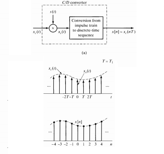
Figure 1. A C/D converter multiplies the input by an impulse train s(t) and generates a discrete-time sequence. Image courtesy of Discrete-Time Signal Processing.
Note that, in Figure 1, xs(t) is still a continuous-time signal; however, x(n) is a discrete-time sequence in which the x-axis is normalized to T.
The Fourier Transform of a Sampled Signal
As shown in Figure 1, during sampling operation, the input is multiplied by an impulse train and we have
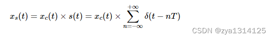
Equation 1
Multiplication in the time domain corresponds to convolution in the frequency domain, and we obtain (Appendix, Equation A1)
Equation 2
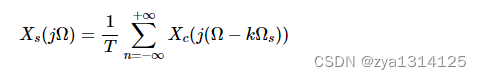
where Ω and Ωs=2π/T denote, respectively, the frequency and the sampling frequency in radians/second. Xs(jΩ) and Xc(jΩ) represent the Fourier transform of xs(t) and xc(t), respectively. Note that Equation 2 gives the Fourier transform of xs(t), not that of x(n); however, for the purpose of this article, we don’t need to know the Fourier transform of x(n). Equation 2 shows an important relation between the Fourier transform of xc(t) and xs(t). According to this equation, if we ignore the scaling factor 1/T, Xs(jΩ) has replicas of Xc(jΩ) at multiples of Ωs. This is illustrated in Figure 2.
Figure 2. Multiplying a signal by an impulse train leads to replicas of the input spectrum at multiples of the sampling frequency. Image courtesy of Discrete-Time Signal Processing.
The Nyquist Sampling Theorem
We want xs(t) to be a representation of xc(t). The question is, can we reconstruct the original continuous-time signal from xs(t)? In other words, given the spectrum in Figure 2(c), can we obtain the frequency domain representation of xc(t) shown in Figure 2(a)?
Figure 2 suggests that we can reconstruct the original signal by applying a low-pass filter to Xs(jΩ) such that the frequency components below ΩN are kept and replicas of Xc(jΩ) at ±Ωs,±2Ωs,…, are removed. However, this is possible only if Ωs−ΩN>ΩN, otherwise, there is no separation between the replicas and we cannot apply the required low-pass filtering. The condition ΩN≤Ωs/2, which is often referred to as the Nyquist sampling theorem, prevents the replicas from overlapping with each other. The mentioned overlapping leads to a kind of distortion called aliasing distortion, or simply aliasing.
To successfully reconstruct xc(t)xc(t) from xs(t), we need xc(t) to be a band-limited signal; otherwise, aliasing will occur. For example, Figure 2(a) shows that Xc(jΩ) has all its energy at Ω<ΩN, i.e., Xc(jΩ)=0 for Ω>ΩN. In practice, xc(t) is not generally a band-limited signal. While we are mainly interested in a particular frequency band of xc(t), there will be strong components or, at least, noise components at frequencies above the desired band. Hence, when sampling with Ωs, we need to place a low-pass filter before the C/D to sufficiently attenuate all the frequency components above Ωs/2. This filter which prevents aliasing is called an anti-aliasing filter.
Minimum Possible Sampling Rate Requires Very Sharp Filters
Suppose that we want to sample an analog music waveform where the desired energy band is in the range 0<|Ω|/2π≤22kHz (Figure 3(a)). According to the Nyquist sampling theorem, the minimum sampling frequency which can be used in this case is 44kHz; however, this requires an anti-aliasing filter with a very steep roll-off. The filter must pass the frequency components from zero to just below 22kHz and reject all the components above 22kHz(Figure 3(b)). The anti-aliasing filter, which is placed before the sampler, is an analog filter and, unfortunately, analog filters cannot achieve a flat passband along with a very sharp transition from passband to stopband. Therefore, in practice, we cannot use a sampling rate of 44kHz for this example.
Combined Analog and Digital Filter
The obvious solution for avoiding the use of a very sharp analog filter will be using a sampling rate higher than 44kHz. For example, suppose that we increase the sampling rate by a factor of 2 and use fs,new=88kHz. In this case, the stopband edge of the anti-aliasing filter will be fs,new/2=44kHz (Figure 3(c)). The passband is still the same as before and we need to pass the frequencies below 22kHz. As a result, the width of the filter’s transition band will be 22kHz, which is practical. Aliasing can be avoided in this way; however, the analog filter will not sufficiently suppress the frequency components from 22kHz to 44kHz, and these unwanted components will enter the system.
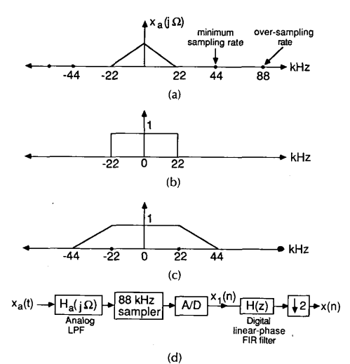
Figure 3. (a) The spectrum of the input signal. (b) The ideal anti-aliasing filter required when using fs=44kHz. (c) Increasing the sample rate relaxes the analog filter requirements. (d) The overall system which uses both analog and digital filtering. Image courtesy of IEEE.
Fortunately, after the ADC, we have the option of using a digital filter (Figure 3(d)), which can offer both sharp transition and linear-phase response. In this way, we can sufficiently suppress the unwanted components from 22kHz to 44kHz.
So far, our system is not a multirate one because there is only one sampling rate used in the system. The overall system obtained from two filters (the analog prefilter and the digital filter) and the analog-to-digital converter is equivalent to that obtained by a sharp analog anti-aliasing filter with passband edge of 22kHz and an ADC sampling at 88 kHz.
But is this system efficient? Do we really need to use 88,000 samples/second to represent a signal that does not have frequency components above 22kHz? Note that after the analog prefilter, there could still be frequency components between 22kHz and 44kHz, but these will be removed by the digital filter. And we know that, according to the Nyquist criterion, we only need 44,000 samples/second to represent our input signal, which has all its energy below 22kHz. This means that we can discard some of the output samples of the above system and still retain all the information we are interested in. Since we want to reduce the sampling rate from 88kHz to 44kHz, we can keep one sample from every two consecutive samples. This operation is called decimation or downsampling (by a factor of 22).
Now there are two sampling rates in our system; before decimation, we were using a sampling rate of 88kHz, and after decimation, the sampling rate is 44kHz. Hence, we have a multirate system. This operation reduces the number of bits used to represent the input signal by a factor of 2. See page 32 of CMOS Integrated Analog-to-Digital and Digital-to-Analog Converters to read about a simple trick which can be used to even further relax the requirements of the analog prefilter in Figure 3(d).
Decimation
A discrete-time sequence x(n) that has been downsampled by a factor of M is given by the following expression:
yd(n)=x(Mn)
This means that we are using only one sample out of every M consecutive samples. In other words, if the sampling rate of x(n) was fs=1/T, the sampling rate of yd(n) will be fs/M. The symbol used for a factor-of-M decimator, and an example of factor-of-2 decimation is illustrated in Figure 4(a), and 4(b), respectively.
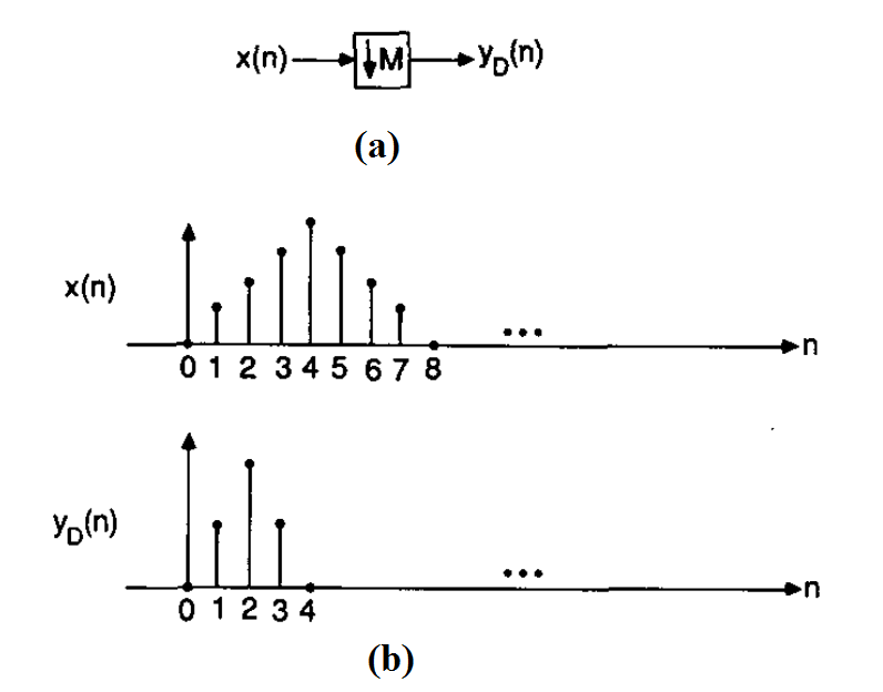
Figure 4. (a) The symbol used for factor-of-M decimation and (b) illustration of factor-of-2 decimation. Image courtesy of IEEE.
Since factor-of-M decimation is equivalent to sampling the underlying analog signal, xc(t), with the sampling rate fs/M, we obtain
yd(n)=xc(nMT)
According to the Nyquist criterion, if xc(t) has frequency components above fs/2M, aliasing will occur. As a result, we usually need to place a low-pass filter with stopband edge frequency of fs/2M before the factor-of-M decimation block. In the example of Figure 3, this filtering task is accomplished by the digital filter that precedes the factor-of-2 decimation stage. The normalized cutoff frequency of this filter will be 2π(fs/2M)*T=π/M. This is illustrated in Figure 5.
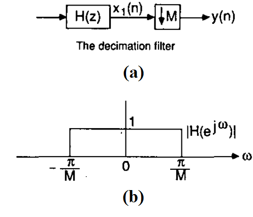
Figure 5. (a) We need a band-limiting filter prior to decimation; (b) the filter used for the factor-of-M decimation. Image courtesy of IEEE.
Appendix
Equation A1


 被折叠的 条评论
为什么被折叠?
被折叠的 条评论
为什么被折叠?
 到【灌水乐园】发言


