Machine Learning Wu Enda3

chapter 27 Multiple features

start to talk about a new version of linear regression,more powerful one that works with multiple variables or with multiple features.

Notation:

n = number of features

$x^{(i)}$ = input (features) of i th training example.

$x_j^{(i)}$ = value of feature j in i th training example.

Hypothesis:

$h_\theta(x) = \theta_0 + \theta_1x_1 + \theta_2x_2 +...+ \theta_nx_n$

for convenience of notation ,define $x_0$ = 1.

$$x= \begin{bmatrix} {x_0}\\ {x_1}\\ {x_2}\\ {\vdots}\\ {x_n}\\ \end{bmatrix} \in \mathbb R^{n+1} \ \ \ \ \ \ \ \ $$
$$\theta= \begin{bmatrix} {\theta_0}\\ {\theta_1}\\ {\theta_2}\\ {\vdots}\\ {\theta_n}\\ \end{bmatrix}\in \mathbb R^{n+1}$$

so

$h_\theta(x) = \theta^Tx$

Multivariate linear regression.

chapter 28 Gradient descent for multiple variables

how to fit the parameters of that hypothesis.how to use gradient descent for linear regression with multiple features

Hypothesis: $h_\theta (x) = \theta^Tx = \theta_0x_0+\theta_1x_1+...+\theta_nx_n)$

Parameters: $\theta$ here is a n+1-dimensional vector.

Cost function:

$J(\theta) = \frac{1}{2m}\sum^m_{i=1}(h_\theta(x^{(i)})-y^{(i)})$

Gradient descent:

​ Repeat{

$\theta_j := \theta_j - a\frac{\partial}{\partial \theta_j}J(\theta)$

​ } (simultaneously update for every $j=0,...,n$)

New algorithm(n>=1):

Repeat{

$\theta_j := \theta_j -a\frac{1}{m}\sum^m_{i=1}(h_\theta(x^{(i)})-y^{(i)})$

}

$\theta_0 := \theta_0 -a\frac{1}{m}\sum^m_{i=1}(h_\theta(x^{(i)})-y^{(i)})x_0^{(i)}$

$\theta_1 := \theta_1 -a\frac{1}{m}\sum^m_{i=1}(h_\theta(x^{(i)})-y^{(i)})x_1^{(i)}$

chapter 29 Gradient descent in practice 1:feature scaling

practical tricks for making gradient descent work well

Feature Scaling:

Idea: Make sure features are on similar scale.

Get every feature into approximately a $-1<= x_i <=1$ range.

Mean normalization

Replace $x_i$ with $x_i-u_i$ to make features have approximately zero mean (Do not apply to $x_0=1$)

$x_1 ← \frac{x_1-u_1}{s_1}$ $u_1$ is the average value of x1 in the training sets.

$s_1$ is the range of values of that feature or standard deviation

chapter 30 Gradient descent in practice 2:learning rate

around the learning rate $a$

• “Debugging “:How to make sure gradient descent is working correctly.
• How to choose learning rate $a$

  

  Declare convergence if $J(\theta)$ decreases by less than $10^{-3}$ in one iteration.

  but choose what this threshold is pretty difficult.So,in order to check your gradient descent has converged, actually tend to look at plots.

  

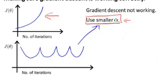
  • For sufficiently small $a$ ,$J(\theta)$should decrease on every iteration.
  • But if $a$ is too small,gradient descent can be slow to converge.
  • if $a$ is too large ;$J(\theta)$ may not decrease on every iteration ;may not converge.

  chapter 31 Features and polynomial regression

  the choice of features that you have and how you can get different learning algorithm

  

  It is important to apply feature scaling if you’re using gradient descent to get them into comparable ranges of values.

  broad choices in the features you use.

  

  chapter 32 Normal equation

  which for some linear regression problems ,will give us a much better way to solve for the optimal value of the parameters $\theta$

  Normal equation : Method to solve for $\theta$ analytically.

  

  

  正规方程推到过程：https://zhuanlan.zhihu.com/p/22474562

  矩阵求导：https://blog.csdn.net/nomadlx53/article/details/50849941

  Gradient Descent and Normal Equation advantages and disadvantages :

  

  The normal equation method actually do not work for those more sophisticated learning algorithms.

  chapter 33 Normal equation and non-invertibility (optional)

  what if $X^TX$ is non-invertible?

  • Redundant features (linearly dependent)

  e g : $x_1$ = size in feet$^2$ $x_2$ = size in m$^2$

  • too many features (e.g m<=n)

  Delete some features , or use regularization.