吴恩达 深度学习 编程作业（1-2）- Python Basics with Numpy & Logistic Regression with a Neural Network mindset

吴恩达Coursera课程 DeepLearning.ai 编程作业系列，本文为《神经网络与深度学习》部分的第二周“神经网络基础”的课程作业（做了无用部分的删减）。

另外，本节课程笔记在此：《吴恩达Coursera深度学习课程 DeepLearning.ai 提炼笔记（1-2）》，如有任何建议和问题，欢迎留言。

---

#Part 1：Python Basics with Numpy (optional assignment)

1 - Building basic functions with numpy

Numpy is the main package for scientific computing in Python. It is maintained by a large community (www.numpy.org). In this exercise you will learn several key numpy functions such as np.exp, np.log, and np.reshape. You will need to know how to use these functions for future assignments.

1.1 - sigmoid function, np.exp()

Exercise: Build a function that returns the sigmoid of a real number x. Use math.exp(x) for the exponential function.

Reminder:
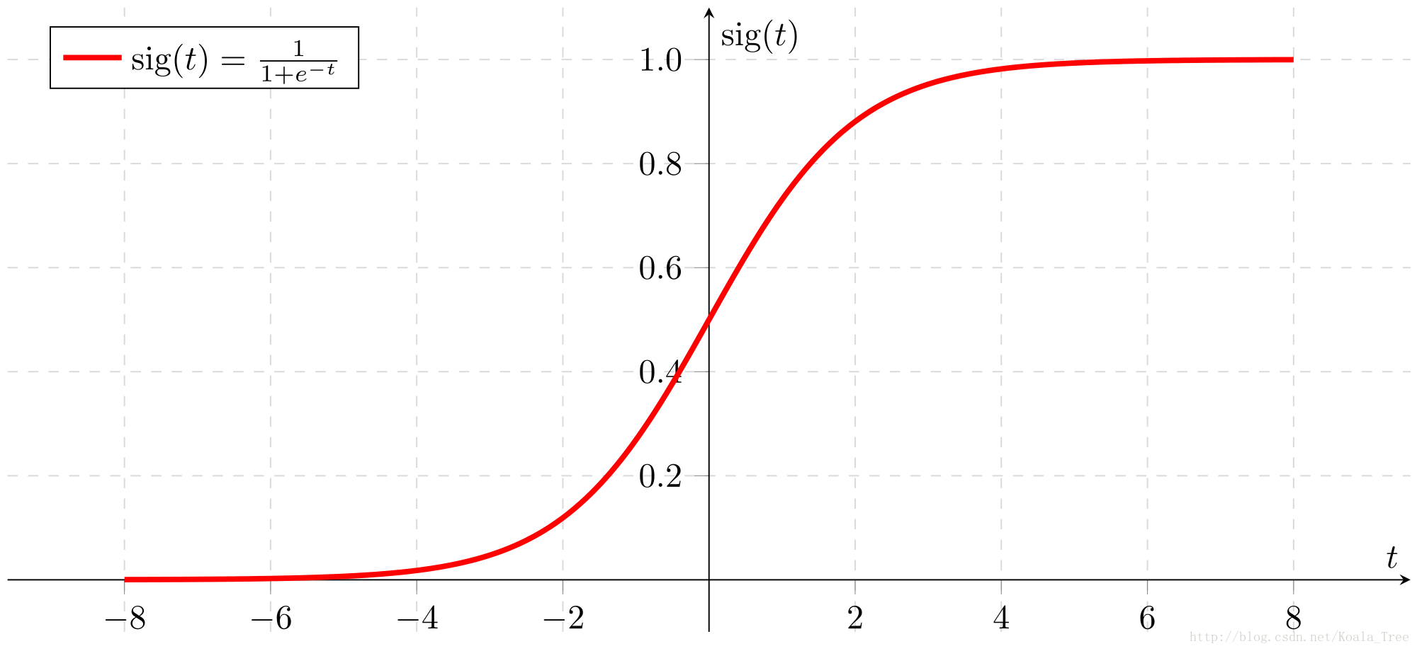
$sigmoid(x)=\frac{1}{1+e^{-x}}$ is sometimes also known as the logistic function. It is a non-linear function used not only in Machine Learning (Logistic Regression), but also in Deep Learning.

To refer to a function belonging to a specific package you could call it using package_name.function(). Run the code below to see an example with math.exp().

# GRADED FUNCTION: basic_sigmoid

import math

def basic_sigmoid(x):
    """
    Compute sigmoid of x.

    Arguments:
    x -- A scalar

    Return:
    s -- sigmoid(x)
    """
    
    ### START CODE HERE ### (≈ 1 line of code)
    s = 1.0 / (1 + 1/ math.exp(x))
    ### END CODE HERE ###
    
    return s

basic_sigmoid(3)

0.9525741268224334

Actually, we rarely use the “math” library in deep learning because the inputs of the functions are real numbers. In deep learning we mostly use matrices and vectors. This is why numpy is more useful.

### One reason why we use "numpy" instead of "math" in Deep Learning ###
x = [1, 2, 3]
basic_sigmoid(x) # you will see this give an error when you run it, because x is a vector.

---------------------------------------------------------------------------

TypeError                                 Traceback (most recent call last)

<ipython-input-3-2e11097d6860> in <module>()
      1 ### One reason why we use "numpy" instead of "math" in Deep Learning ###
      2 x = [1, 2, 3]
----> 3 basic_sigmoid(x) # you will see this give an error when you run it, because x is a vector.


<ipython-input-1-65a96864f65f> in basic_sigmoid(x)
     15 
     16     ### START CODE HERE ### (≈ 1 line of code)
---> 17     s = 1.0 / (1 + 1/ math.exp(x))
     18     ### END CODE HERE ###
     19 


TypeError: a float is required

In fact, if $ x = (x_1, x_2, …, x_n)$ is a row vector then $np.exp(x)$ will apply the exponential function to every element of x. The output will thus be: $np.exp(x)=(e^{x_1},e^{x_2},...,e^{x_n})$

import numpy as np

# example of np.exp
x = np.array([1, 2, 3])
print(np.exp(x)) # result is (exp(1), exp(2), exp(3))

[  2.71828183   7.3890561   20.08553692]

Furthermore, if x is a vector, then a Python operation such as $s=x+3$ or $s=\frac{1}{x}$ will output s as a vector of the same size as x.

# example of vector operation
x = np.array([1, 2, 3])
print (x + 3)

[4 5 6]

Exercise: Implement the sigmoid function using numpy.

Instructions: x could now be either a real number, a vector, or a matrix. The data structures we use in numpy to represent these shapes (vectors, matrices…) are called numpy arrays. You don’t need to know more for now.
$$\text{For }x\in {\mathbb{R}}^n\text{, }sigmoid(x)=sigmoid\left(\begin{array}{c}{x}_1\\ x_2\\ ...\\ x_n\end{array}\right)=\left(\begin{array}{c}\frac{1}{1+e^{-x_1}}\\ \frac{1}{1+e^{-x_2}}\\ ...\\ \frac{1}{1+e^{-x_n}}\end{array}\right)\text{\hspace{1em}(1)}$$

# GRADED FUNCTION: sigmoid

import numpy as np # this means you can access numpy functions by writing np.function() instead of numpy.function()

def sigmoid(x):
    """
    Compute the sigmoid of x

    Arguments:
    x -- A scalar or numpy array of any size

    Return:
    s -- sigmoid(x)
    """
    
    ### START CODE HERE ### (≈ 1 line of code)
    s = 1.0 / (1 + 1 / np.exp(x))
    ### END CODE HERE ###
    
    return s

x = np.array([1, 2, 3])
sigmoid(x)

array([ 0.73105858,  0.88079708,  0.95257413])

1.2 - Sigmoid gradient

Exercise: Implement the function sigmoid_grad() to compute the gradient of the sigmoid function with respect to its input x. The formula is: $$sigmoid\_derivative(x)={\sigma }^{\prime }(x)=\sigma (x)(1-\sigma (x))\text{\hspace{1em}(2)}$$
You often code this function in two steps:

1. Set s to be the sigmoid of x. You might find your sigmoid(x) function useful.
2. Compute ${\sigma }^{\prime }(x)=s(1-s)$

# GRADED FUNCTION: sigmoid_derivative

def sigmoid_derivative(x):
    """
    Compute the gradient (also called the slope or derivative) of the sigmoid function with respect to its input x.
    You can store the output of the sigmoid function into variables and then use it to calculate the gradient.
    
    Arguments:
    x -- A scalar or numpy array

    Return:
    ds -- Your computed gradient.
    """
    
    ### START CODE HERE ### (≈ 2 lines of code)
    s = 1.0 / (1 + 1 / np.exp(x))
    ds = s * (1 - s)
    ### END CODE HERE ###
    
    return ds

x = np.array([1, 2, 3])
print ("sigmoid_derivative(x) = " + str(sigmoid_derivative(x)))

sigmoid_derivative(x) = [ 0.19661193  0.10499359  0.04517666]

1.3 - Reshaping arrays

Two common numpy functions used in deep learning are np.shape and np.reshape().

• X.shape is used to get the shape (dimension) of a matrix/vector X.
• X.reshape(…) is used to reshape X into some other dimension.

For example, in computer science, an image is represented by a 3D array of shape $(length,height,depth=3)$. However, when you read an image as the input of an algorithm you convert it to a vector of shape $(length\ast height\ast 3,1)$. In other words, you “unroll”, or reshape, the 3D array into a 1D vector.

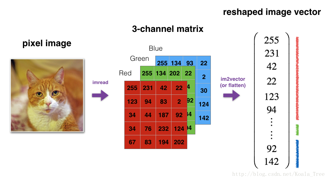
Exercise: Implement image2vector() that takes an input of shape (length, height, 3) and returns a vector of shape (length*height*3, 1). For example, if you would like to reshape an array v of shape (a, b, c) into a vector of shape (a*b,c) you would do:

v = v.reshape((v.shape[0]*v.shape[1], v.shape[2])) # v.shape[0] = a ; v.shape[1] = b ; v.shape[2] = c

• Please don’t hardcode the dimensions of image as a constant. Instead look up the quantities you need with image.shape[0], etc.

# GRADED FUNCTION: image2vector
def image2vector(image):
    """
    Argument:
    image -- a numpy array of shape (length, height, depth)
    
    Returns:
    v -- a vector of shape (length*height*depth, 1)
    """
    
    ### START CODE HERE ### (≈ 1 line of code)
    v = image.reshape((image.shape[0] * image.shape[1] * image.shape[2], 1))
    ### END CODE HERE ###
    
    return v

# This is a 3 by 3 by 2 array, typically images will be (num_px_x, num_px_y,3) where 3 represents the RGB values
image = np.array([[[ 0.67826139,  0.29380381],
        [ 0.90714982,  0.52835647],
        [ 0.4215251 ,  0.45017551]],

       [[ 0.92814219,  0.96677647],
        [ 0.85304703,  0.52351845],
        [ 0.19981397,  0.27417313]],

       [[ 0.60659855,  0.00533165],
        [ 0.10820313,  0.49978937],
        [ 0.34144279,  0.94630077]]])

print ("image2vector(image) = " + str(image2vector(image)))

image2vector(image) = [[ 0.67826139]
 [ 0.29380381]
 [ 0.90714982]
 [ 0.52835647]
 [ 0.4215251 ]
 [ 0.45017551]
 [ 0.92814219]
 [ 0.96677647]
 [ 0.85304703]
 [ 0.52351845]
 [ 0.19981397]
 [ 0.27417313]
 [ 0.60659855]
 [ 0.00533165]
 [ 0.10820313]
 [ 0.49978937]
 [ 0.34144279]
 [ 0.94630077]]

1.4 - Normalizing rows

Another common technique we use in Machine Learning and Deep Learning is to normalize our data. It often leads to a better performance because gradient descent converges faster after normalization. Here, by normalization we mean changing x to $ \frac{x}{| x|} $ (dividing each row vector of x by its norm).

For example, if $$x=\left[\begin{array}{ccc}0& 3& 4\\ 2& 6& 4\end{array}\right]\text{\hspace{1em}(3)}$$ then $$\Vert x\Vert =np.linalg.norm(x,axis=1,keepdims=True)=[\begin{array}{c}5\\ \sqrt{56}\end{array}$$