[ESL] Chapter 2(一)

Figure 2.1 - 2.5

Figure 2.1

######################generate mixture Gaussian#############

library(MASS)
# generate means of mixture Gaussian
blueMeans <- mvrnorm(10, c(1,0), diag(2))
redMeans <- mvrnorm(10, c(0,1), diag(2))
allMeans <- rbind(blueMeans, redMeans)

# generate mixture Gaussian
blueData <- mvrnorm(100, c(0,0), diag(2)/5) + blueMeans[sample(1:10, 100, replace=TRUE),]
redData <- mvrnorm(100, c(0,0), diag(2)/5) + redMeans[sample(1:10, 100, replace=TRUE),]

# combind data 
x <- rbind(blueData, redData)
y <- c(rep(0,100), rep(1,100))

#################linear regression for classification#######

# fit linear regression
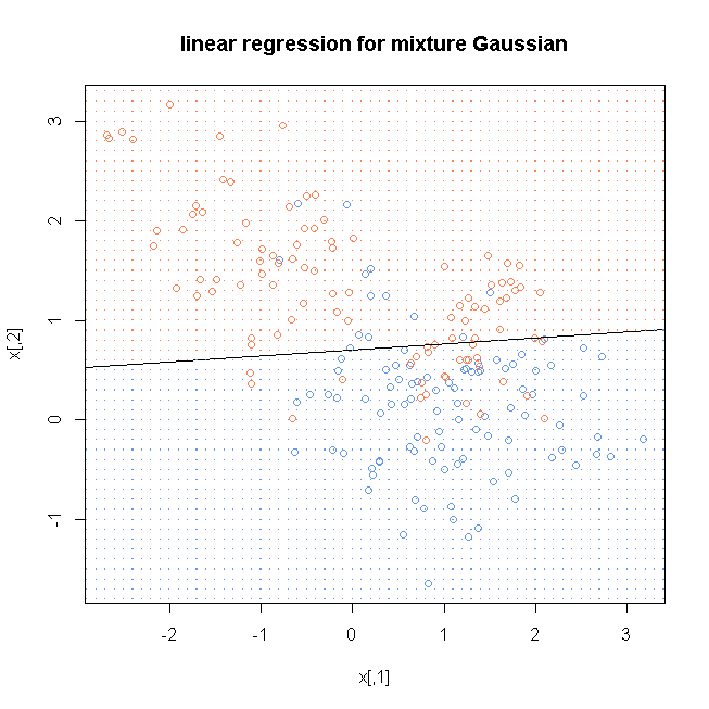
lmfit <- lm(y~., data=as.data.frame(x))

# get coefficient of lmfit
lmcoef <- coef(lmfit)

#plot figure 2.1
## plot data
windows()
plot(x, col=ifelse(y==0, "cornflowerblue", "coral"), main="linear regression for mixture Gaussian")
## line lmfit on plot
abline((-lmcoef[1]+0.5)/lmcoef[3], -lmcoef[2]/lmcoef[3])

# generate grid data
x1 <- seq(floor(min(x[,1])), ceiling(max(x[,1])), by=0.1)
x2 <- seq(floor(min(x[,2])), ceiling(max(x[,2])), by=0.1)

xnew <- cbind(rep(x1, length(x2)), rep(x2, each=length(x1)))

# predict xnew using lmfit
yhat <- predict(lmfit, as.data.frame(xnew))

# point grid data on plot
dg <- expand.grid(x=x1, y=x2)
points(dg, pch=".", cex=1.2, col=ifelse(yhat>0.5, "coral", "cornflowerblue"))
box()

Figure 2.2

#############Figure 2.2: 15-nearest neighbors section#######

# predict on xnew using parallel
# generate mixture gaussian data with parallel
library(class)
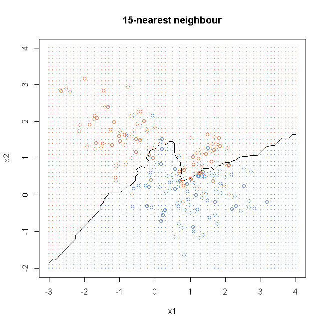
result15<- knn(x, xnew, y, k=15, prob=TRUE)
prob15 <- attr(result15, "prob")
prob15 <- ifelse(result15=="1", prob15, 1-prob15)
probMat <- matrix(prob15, nrow = length(x1))

# plot data
windows()
plot(x, col=ifelse(y==0, "cornflowerblue", "coral"), xaxt = "n", yaxt = "n", ann = FALSE)

# plot the separation boundary
contour(x1, x2, probMat, levels=0.5, labels="", xlab="x1", ylab="x2", main="15-nearest neighbour")

# points the data on the plot
points(x, col=ifelse(y==0, "cornflowerblue", "coral"))

# adding grid
gd <- expand.grid(x=x1, y=x2)
points(gd, pch=".", cex=1.2, col=ifelse(prob15>0.5, "coral", "cornflowerblue"))
box()

Figure 2.3

#############Figure 2.3: 1-nearest neighbors section#######

# predict on xnew using parallel
# generate mixture gaussian data with parallel
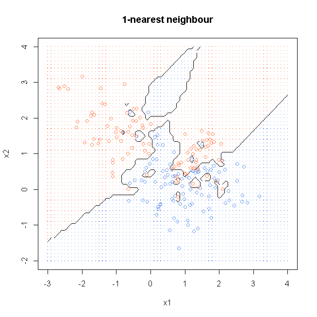
result1<- knn(x, xnew, y, k=1, prob=TRUE)
prob1 <- attr(result1, "prob")
prob1 <- ifelse(result1=="1", prob1, 1-prob1)
probMat <- matrix(prob1, nrow = length(x1))

# plot data
windows()
plot(x, col=ifelse(y==0, "cornflowerblue", "coral"), xaxt = "n", yaxt = "n", ann = FALSE)

# plot the separation boundary
contour(x1, x2, probMat, levels=0.5, labels="", xlab="x1", ylab="x2", main="1-nearest neighbour")

# points the data on the plot
points(x, col=ifelse(y==0, "cornflowerblue", "coral"))

# adding grid
gd <- expand.grid(x=x1, y=x2)
points(gd, pch=".", cex=1.2, col=ifelse(prob1>0.5, "coral", "cornflowerblue"))
box()

Figure 2.4

#############train and test error#########################

# generate test data
centers <- c(sample(1:10, 5000, replace=TRUE), 
             sample(11:20, 5000, replace=TRUE))
means <- allMeans[centers, ]
xTest <- mvrnorm(10000, c(0,0), 0.2*diag(2)) + means
yTest <- c(rep(0, 5000), rep(1, 5000))

# train and test error
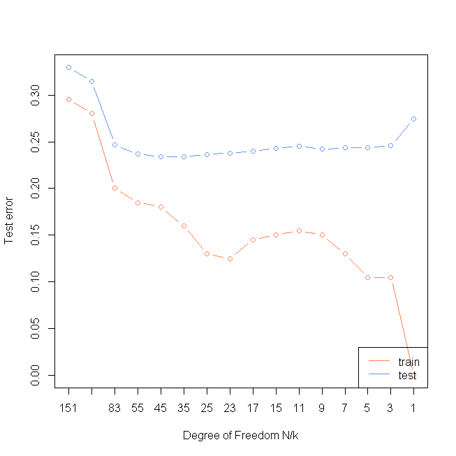
ks <- c(1,3,5,7,9,11,15,17,23,25,35,45,55,83,101,151 )
misTrain <- rep(0, length(ks))
misTest <- rep(0, length(ks))
for(i in 1:length(ks)){
  preTrain <- knn(x, x, y, k=ks[i])
  preTest <- knn(x, xTest, y, k=ks[i])
  misTrain[i] <- sum(preTrain!=y)/length(y)
  misTest[i] <- sum(preTest!=yTest)/length(yTest)
}

# plot 
windows()
plot(rev(misTrain), col="coral", xlab="Degree of Freedom N/k",ylab="Test error",type="n",xaxt="n", ylim=c(0, max(misTest)))
axis(1, rev(1:length(ks)), as.character(ks))
lines(rev(misTest), type="b", col="cornflowerblue")
lines(rev(misTrain), type="b", col="coral")
legend("bottomright", lty=1, col=c("coral", "cornflowerblue"), legend = c("train ", "test "))

Figure 2.5

###################bayes boundary###########################
library(mvtnorm)
# each column correspondint to a mean: blue class
bayesBlueMat <- apply(blueMeans, 1, function(z)dmvnorm(xnew, z, diag(2)/5))
# bayes probability
bayesBlueProb <- apply(bayesBlueMat, 1, mean)

# each column correspondint to a mean: red
bayesRedMat <- apply(redMeans, 1, function(z)dmvnorm(xnew, z, diag(2)/5))
# bayes probability
bayesRedProb <- apply(bayesRedMat, 1, mean)

# bayes prob of two class
bayesProb <- cbind(bayesBlueProb, bayesRedProb)
# bayes class
bayesLabel <- t(apply(bayesProb, 1, order))[,2]
# prob of win class
bayesWinProb <- apply(bayesProb, 1, max)
bayesProb1 <- ifelse(bayesLabel==1, bayesWinProb, 1-bayesWinProb)
bayesGridMat <- matrix(bayesProb1, nrow=length(x1))

# plot data
windows()
plot(x, col=ifelse(y==0, "cornflowerblue", "coral"), xaxt = "n", yaxt = "n", ann = FALSE)

# plot the separation boundary
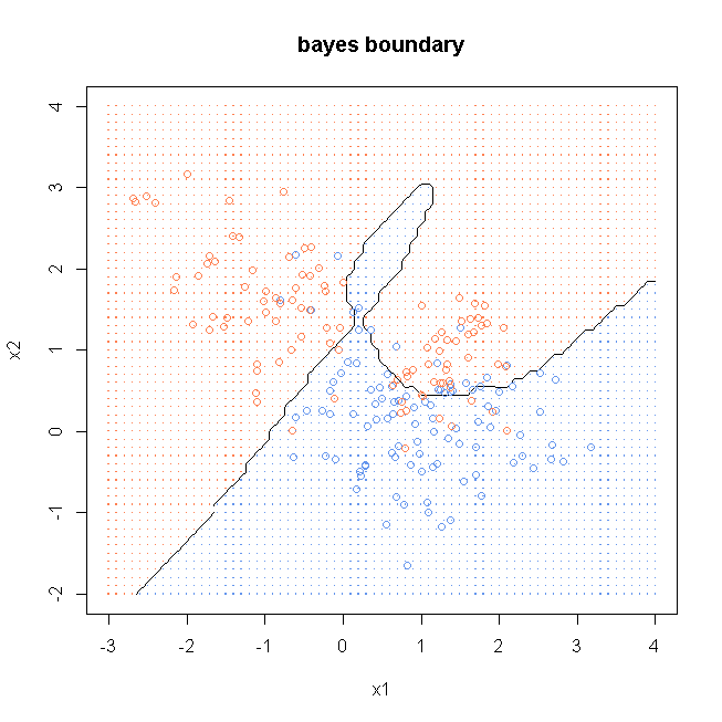
contour(x1, x2, bayesGridMat, levels=0.5, labels="", xlab="x1", ylab="x2", main="bayes boundary")

# points the data on the plot
points(x, col=ifelse(y==0, "cornflowerblue", "coral"))

# adding grid
gd <- expand.grid(x=x1, y=x2)
points(gd, pch=".", cex=1.2, col=ifelse(bayesProb1>0.5, "coral", "cornflowerblue"))
box()