Notes on Convolutional Neural Networks（阅读）

这篇文章是大家熟悉的CNN，这是被埋没了很久的一篇，是金子总会发光。网络测试的可视化效果，http://yann.lecun.com/exdb/lenet/index.html

=====================================================================

使用的代码：DeepLearnToolbox  ，下载地址：点击打开，感谢该toolbox的作者

=====================================================================

大家经常看的大牛博客讲解系列的介绍http://blog.csdn.net/zouxy09。虽然已经很详细了，总归自己要看一下原文，CNN的matlab代码已经详细跑过一次了，里面的参数变化图片变化都已经实现了。这里总结一下。

一、Feedforward Pass

（公式是平方误差损失函数，c是多少类，N是样本数，t的角标意思是第n个样本的第k维对应的label，y的角标意思是第n个样本第k维的输出）

（l为当前所在层数，f为我前面文章中介绍的激活函数，这里不详细说明了，b为偏置（经常会提到权值共享，同一平面层的神经元权值相同，不同map的权值不共享），w是核吧，x是神经元）。

二·、Backpropagation Pass

（这是前L层的灵敏度也就是残差）

（输出层L的灵敏度）

（每一个权值(W)_ij都有一个特定的学习率η_Ij）

关于反向传导的推导http://blog.csdn.net/langb2014/article/details/46670901的第二部分推导，之前很详细的整理过。

三、Convolution Layers

1、Computing the Gradients

up(.)表示一个上采样操作。如果下采样的采样因子是n的话，它简单的将每个像素水平和垂直方向上拷贝n次。

_（是中的在卷积的时候与逐元素相乘的patch，输出卷积map的(u, v)位置的值是由上一层的(u, v)位置的patch与卷积核k_ij逐元素相乘的结果。_）

四、Sub-sampling Layers

1、Computing the Gradients

b和β计算梯度:

五、Learning Combinations of Feature Maps

条件：

softmax：

六、Enforcing Sparse Combinations

稀疏方面的正则项之前介绍过了；

这是原《Notes on Convolutional Neural Networks》的大概公式流程，感觉非常乱。

====================================================================

整个流程梳理一下：

CNN的基本结构大概就是这样，由输入、卷积层、子采样层、全连接层、分类层、输出组成。

斯坦福在线教程很详细http://ufldl.stanford.edu/tutorial/supervised/ConvolutionalNeuralNetwork/

 

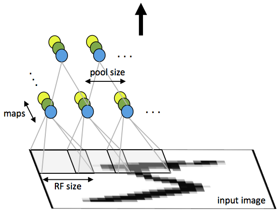
Fig 1: First layer of a convolutional neural network with pooling. Units of the same color have tied weights and units of different color represent different filter maps.

1、卷积过程

 

2、pooling过程

3、SGD的实现：http://blog.csdn.net/langb2014/article/details/48262303

使用带动量项的梯度下降法SGD：

（在我前面的alexnet中第九部分说明了一下http://blog.csdn.net/langb2014/article/details/48286501）

4、softmax分类层：

中文介绍相信大家都能看懂http://ufldl.stanford.edu/wiki/index.php/Softmax%E5%9B%9E%E5%BD%92

=====================================================================

教程中

 第一点，梯度检验对求导结果进行数值检验，EPSILON不能太小，它给出一个0.0001，说是一个范围，也就是0.01~0.001~0.0001~0.00001甚至跟小都可以。

第二点：Debugging: Bias and Variance

Bias: a learner’s tendency to consistently learn the same wrong thing，即度量了某种学习算法的平均估计结果所能逼近学习目标(目标输出)的程度。

Variance：the tendency to learn random things irrespective of the real signal，即度量了在面对同样规模的不同训练集时，学习算法的估计结果发生变动的程度。比如在同一现象所产生的不同训练数据上学习的决策树往往差异巨大，而实际上它们应当是相同的。

从图像角度

靶心为某个能完美预测的模型，离靶心越远，则准确率随之降低。靶上的点代表某次对某个数据集上学习某个模型。纵向上，高低的bias：高的Bias表示离目标较远，低bias表示离靶心越近；横向上，高低的variance，高的variance表示多次的“学习过程”越分散，反之越集中。

从数学定义角度

以分类任务为例，均方误差MSE（mean squared error）

，其中Y为x对应的真实类标，f(x)为预测标号

则，

所以bias表示预测值的均值与实际值的差值；而variance表示预测结果作为一个随机变量时的方差。

Bias、variance与复杂度的关系

第三点：Debugging: Optimizers and Objectives

  （1）滤波器的数量选择：在选定每一层的滤波器的数量的时候，要牢记计算一个卷积层滤波器的激活函数比计算传统的MLPs的激活函数的代价要高很多！假设第（i-1）层包含了Ki-1个特征图和M*N个像素坐标（如坐标位置数目乘以特征图数目），在l层有Kl个m*n的滤波器，所以计算特征图的代价为：（M-m）*（N-n）*m*n*Kl-1。整个代价是Kl乘级的。如果一层的所有特征图没有和前一层的所有的特征图全部连起来，情况可能会更加复杂一些。对于标准的MLP，这个代价为Kl * Kl-1，Kl是第l层上的不同的节点。所以，CNNs中的特征图数目一般比MLPs中的隐层节点数目要少很多，这还取决于特征图的尺寸大小。因为特征图的尺寸随着层次深度的加大而变小，越靠近输入，所在层所包含的特征图越少，高层的特征图会越多。实际上，把每一次的计算平均一下，输出的特征图的的数目和像素位置的数目在各层是大致保持不变的。To preserve the information about the input would require keeping the total number of activations (number of feature maps times number of pixel positions) to be non-decreasing from one layer to the next (of

course we could hope to get away with less when we are doing supervised learning).所以特征图的数量直接控制着模型的容量，它依赖于样本的数量和任务的复杂度。

  （2）滤波器的模型属性(shape)：一般来说，在论文中，由于所用的数据库不一样，滤波器的模型属性变化都会比较大。最好的CNNs的MNIST分类结果中，图像（28*28）在第一层的输入用的5*5的窗口（感受野），然后自然图像一般都使用更大的窗口，如12*12,15*15等。为了在给定数据库的情况下，获得某一个合适的尺度下的特征，需要找到一个合适的粒度等级。

  （3）最大池化的模型属性：典型的取值是2*2或者不用最大池化。比较大的图像可以在CNNs的低层用4*4的池化窗口。但是要需要注意的是，这样的池化在降维的同事也有可能导致信息丢失严重。

  （4）注意点：如果想在一些新的数据库上用CNN进行测试，可以对数据先进行白化处理（如用PCA），还有就是在每次训练迭代中减少学习率，这样可能会得到更好的实验效果。

=====================================================================

CNN困惑的地方：主要遇到各维度参数调节问题。

具体如下：
1.CNN的深度层数参数，即应该设定多少层？这个参数应该怎么确定？相关的层类型顺序需不需要太多的讲究？（比如设定为：卷积层，卷积层，采样层，全连接层之类）
2.CNN的神经元数目参数，即在上述1参数确定条件下，每层应该选多少神经元数目？
3.CNN的卷积核大小参数，即应该选定多大维度（m*n）的卷积核进行卷积？
4.CNN的权重W矩阵，即怎么确定W？完全根据训练集误差最小得到W感觉效果不好，所以我现在利用交叉验证集的拐点位置定W（防止过拟合），不知道是否有问题？
解决的方法如下（总体效果不是很好）：
a.针对上述1问题，利用“经验性”的做法（即简单手动试了几组）简单确定了5层（即2层卷积层，1层采样层，2层全连接层）；即没有严格调节训练该参数的过程。
b.针对上述2问题，也是利用了“经验性”的做法简单确定神经元的数目（不过根据Andrew Ng讲的课，我让神经元数目 处于略多的趋势，然后加了正则化的处理方法）。
c.针对上述3问题，根据我们具体的数据背景含义，手动的选了相应的卷积核大小。

总的来说，处理的过程是符合机器学习处理的一般过程，分成3堆数据集（训练，交叉，测试），用交叉集的拐点确定W和正则化值lamda，测试集报预测率，平均预测率只有72%左右。

=====================================================================

Hinton亲传弟子Ilya Sutskever的深度学习综述及实际建议(原文很长很长，只节选practical advice部分)            

         --------------------http://yyue.blogspot.jp/2015/01/a-brief-overview-of-deep-learning.html

Here is a summary of the community’s knowledge of what’s important and what to look after:

• Get the data: Make sure that you have a high-quality dataset of input-output examples that is large, representative, and has relatively clean labels. Learning is completely impossible without such a dataset.
  
• Preprocessing: it is essential to center the data so that its mean is zero and so that the variance of each of its dimensions is one. Sometimes, when the input dimension varies by orders of magnitude, it is better to take the log(1 + x) of that dimension. Basically, it’s important to find a faithful encoding of the input with zero mean and sensibly bounded dimensions. Doing so makes learning work much better. This is the case because the weights are updated by the formula: change in w_ij \propto x_idL/dy_j (w denotes the weights from layer x to layer y, and L is the loss function). If the average value of the x’s is large (say, 100), then the weight updates will be very large and correlated, which makes learning bad and slow. Keeping things zero-mean and with small variance simply makes everything work much better.
  
• Minibatches: Use minibatches. Modern computers cannot be efficient if you process one training case at a time. It is vastly more efficient to train the network on minibatches of 128 examples, because doing so will result in massively greater throughput. It would actually be nice to use minibatches of size 1, and they would probably result in improved performance and lower overfitting; but the benefit of doing so is outweighed the massive computational gains provided by minibatches. But don’t use very large minibatches because they tend to work less well and overfit more. So the practical recommendation is: use the smaller minibatch that runs efficiently on your machine.
  
• Gradient normalization: Divide the gradient by minibatch size. This is a good idea because of the following pleasant property: you won’t need to change the learning rate (not too much, anyway), if you double the minibatch size (or halve it).
  
• Learning rate schedule: Start with a normal-sized learning rate (LR) and reduce it towards the end.
  
  • A typical value of the LR is 0.1. Amazingly, 0.1 is a good value of the learning rate for a large number of neural networks problems. Learning rates frequently tend to be smaller but rarely much larger.
  • Use a validation set ---- a subset of the training set on which we don’t train --- to decide when to lower the learning rate and when to stop training (e.g., when error on the validation set starts to increase).
  • A practical suggestion for a learning rate schedule: if you see that you stopped making progress on the validation set, divide the LR by 2 (or by 5), and keep going. Eventually, the LR will become very small, at which point you will stop your training. Doing so helps ensure that you won’t be (over-)fitting the training data at the detriment of validation performance, which happens easily and often. Also, lowering the LR is important, and the above recipe provides a useful approach to controlling via the validation set.
  
  
• But most importantly, worry about the Learning Rate. One useful idea used by some researchers (e.g.,Alex Krizhevsky) is to monitor the ratio between the update norm and the weight norm. This ratio should be at around 10^-3. If it is much smaller then learning will probably be too slow, and if it is much larger then learning will be unstable and will probably fail.
  
• Weight initialization. Worry about the random initialization of the weights at the start of learning.
  
  • If you are lazy, it is usually enough to do something like 0.02 * randn(num_params). A value at this scale tends to work surprisingly well over many different problems. Of course, smaller (or larger) values are also worth trying.
  • If it doesn’t work well (say your neural network architecture is unusual and/or very deep), then you should initialize each weight matrix with the init_scale / sqrt(layer_width) * randn. In this case init_scale should be set to 0.1 or 1, or something like that.
  • Random initialization is super important for deep and recurrent nets. If you don’t get it right, then it’ll look like the network doesn’t learn anything at all. But we know that neural networks learn once the conditions are set.
  • Fun story: researchers believed, for many years, that SGD cannot train deep neural networks from random initializations. Every time they would try it, it wouldn’t work. Embarrassingly, they did not succeed because they used the “small random weights” for the initialization, which works great for shallow nets but simply doesn’t work for deep nets at all. When the nets are deep, the many weight matrices all multiply each other, so the effect of a suboptimal scale is amplified.
  • But if your net is shallow, you can afford to be less careful with the random initialization, since SGD will just find a way to fix it.
  You’re now informed. Worry and care about your initialization. Try many different kinds of initialization. This effort will pay off. If the net doesn’t work at all (i.e., never “gets off the ground”), keep applying pressure to the random initialization. It’s the right thing to do.
  
• If you are training RNNs or LSTMs, use a hard constraint over the norm of the gradient (remember that the gradient has been divided by batch size). Something like 15 or 5 works well in practice in my own experiments. Take your gradient, divide it by the size of the minibatch, and check if its norm exceeds 15 (or 5). If it does, then shrink it until it is 15 (or 5). This one little trick plays a huge difference in the training of RNNs and LSTMs, where otherwise the exploding gradient can cause learning to fail and force you to use a puny learning rate like 1e-6 which is too small to be useful.
  
• Numerical gradient checking: If you are not using Theano or Torch, you’ll be probably implementing your own gradients. It is easy to make a mistake when we implement a gradient, so it is absolutely critical to use numerical gradient checking. Doing so will give you a complete peace of mind and confidence in your code. You will know that you can invest effort in tuning the hyperparameters (such as the learning rate and the initialization) and be sure that your efforts are channeled in the right direction.
  
• If you are using LSTMs and you want to train them on problems with very long range dependencies, you should initialize the biases of the forget gates of the LSTMs to large values. By default, the forget gates are the sigmoids of their total input, and when the weights are small, the forget gate is set to 0.5, which is adequate for some but not all problems. This is the one non-obvious caveat about the initialization of the LSTM.
  
• Data augmentation: be creative, and find ways to algorithmically increase the number of training cases that are in your disposal. If you have images, then you should translate and rotate them; if you have speech, you should combine clean speech with all types of random noise; etc. Data augmentation is an art (unless you’re dealing with images). Use common sense.
  
• Dropout. Dropout provides an easy way to improve performance. It’s trivial to implement and there’s little reason to not do it. Remember to tune the dropout probability,and to not forget to turn off Dropout and to multiply the weights by (namely by 1-dropout probability)at test time. Also, be sure to train the network for longer. Unlike normal training, where the validation error often starts increasing after prolonged training, dropout nets keep getting better and better the longer you train them. So be patient.
  
• Ensembling. Train 10 neural networks and average their predictions. It’s a fairly trivial technique that results in easy, sizeable performance improvements. One may be mystified as to why averaging helps so much, but there is a simple reason for the effectiveness of averaging. Suppose that two classifiers have an error rate of 70%. Then, when they agree they are right. But when they disagree, one of them is often right, so now the average prediction will place much more weight on the correct answer. The effect will be especially strong whenever the network is confident when it’s right and unconfident when it’s wrong.

I am pretty sure that I haven’t forgotten anything. The above 13 points cover literally everything that’s needed in order to train LDNNs successfully.

=====================================================================

经验值？因为听好多大神说调参数都是什么经验值，其实不全是这个原因，然后大神推荐看一下一本书

<Neural Networks Tricks of the Trade>这本书综述了神经网络各种trick，人家大神多年调参总结出的各种tricks。下面是电子稿链接:http://pan.baidu.com/s/1pJ9WUvh 密码: b5b2

=====================================================================

matlab代码分解：

cnnexamples.m

clear all; close all; clc;
addpath('../data');
addpath('../util');
load mnist_uint8;

train_x = double(reshape(train_x',28,28,60000))/255;
test_x = double(reshape(test_x',28,28,10000))/255;
train_y = double(train_y');
test_y = double(test_y');

%% ex1 
%will run 1 epoch in about 200 second and get around 11% error. 
%With 100 epochs you'll get around 1.2% error

cnn.layers = {
    struct('type', 'i') %input layer
    struct('type', 'c', 'outputmaps', 6, 'kernelsize', 5) %convolution layer
    struct('type', 's', 'scale', 2) %sub sampling layer
    struct('type', 'c', 'outputmaps', 12, 'kernelsize', 5) %convolution layer
    struct('type', 's', 'scale', 2) %subsampling layer
};

% 这里把cnn的设置给cnnsetup，它会据此构建一个完整的CNN网络，并返回
cnn = cnnsetup(cnn, train_x, train_y);

% 学习率
opts.alpha = 1;
% 每次挑出一个batchsize的batch来训练，也就是每用batchsize个样本就调整一次权值，而不是
% 把所有样本都输入了，计算所有样本的误差了才调整一次权值
opts.batchsize = 50; 
% 训练次数，用同样的样本集。我训练的时候：
% 1的时候 11.41% error
% 5的时候 4.2% error
% 10的时候 2.73% error
opts.numepochs = 10;

% 然后开始把训练样本给它，开始训练这个CNN网络
cnn = cnntrain(cnn, train_x, train_y, opts);

% 然后就用测试样本来测试
[er, bad] = cnntest(cnn, test_x, test_y);

%plot mean squared error
plot(cnn.rL);
%show test error
disp([num2str(er*100) '% error']);

cnnsetup.m

function net = cnnsetup(net, x, y)
    inputmaps = 1;
	% B=squeeze(A) 返回和矩阵A相同元素但所有单一维都移除的矩阵B，单一维是满足size(A,dim)=1的维。
	% train_x中图像的存放方式是三维的reshape(train_x',28,28,60000)，前面两维表示图像的行与列，
	% 第三维就表示有多少个图像。这样squeeze(x(:, :, 1))就相当于取第一个图像样本后，再把第三维
	% 移除，就变成了28x28的矩阵，也就是得到一幅图像，再size一下就得到了训练样本图像的行数与列数了
    mapsize = size(squeeze(x(:, :, 1)));

	% 下面通过传入net这个结构体来逐层构建CNN网络
	% n = numel(A)返回数组A中元素个数
	% net.layers中有五个struct类型的元素，实际上就表示CNN共有五层，这里范围的是5
    for l = 1 : numel(net.layers)   %  layer
        if strcmp(net.layers{l}.type, 's') % 如果这层是 子采样层
            % subsampling层的mapsize，最开始mapsize是每张图的大小28*28
			% 这里除以scale=2，就是pooling之后图的大小，pooling域之间没有重叠，所以pooling后的图像为14*14
			% 注意这里的右边的mapsize保存的都是上一层每张特征map的大小，它会随着循环进行不断更新
			mapsize = floor(mapsize / net.layers{l}.scale);
            for j = 1 : inputmaps % inputmap就是上一层有多少张特征图
                net.layers{l}.b{j} = 0; % 将偏置初始化为0
            end
        end
        if strcmp(net.layers{l}.type, 'c') % 如果这层是 卷积层
            % 旧的mapsize保存的是上一层的特征map的大小，那么如果卷积核的移动步长是1，那用
			% kernelsize*kernelsize大小的卷积核卷积上一层的特征map后，得到的新的map的大小就是下面这样
			mapsize = mapsize - net.layers{l}.kernelsize + 1;
			% 该层需要学习的参数个数。每张特征map是一个(后层特征图数量)*(用来卷积的patch图的大小)
			% 因为是通过用一个核窗口在上一个特征map层中移动（核窗口每次移动1个像素），遍历上一个特征map
			% 层的每个神经元。核窗口由kernelsize*kernelsize个元素组成，每个元素是一个独立的权值，所以
			% 就有kernelsize*kernelsize个需要学习的权值，再加一个偏置值。另外，由于是权值共享，也就是
			% 说同一个特征map层是用同一个具有相同权值元素的kernelsize*kernelsize的核窗口去感受输入上一
			% 个特征map层的每个神经元得到的，所以同一个特征map，它的权值是一样的，共享的，权值只取决于
			% 核窗口。然后，不同的特征map提取输入上一个特征map层不同的特征，所以采用的核窗口不一样，也
			% 就是权值不一样，所以outputmaps个特征map就有（kernelsize*kernelsize+1）* outputmaps那么多的权值了
			% 但这里fan_out只保存卷积核的权值W，偏置b在下面独立保存
            fan_out = net.layers{l}.outputmaps * net.layers{l}.kernelsize ^ 2;
            for j = 1 : net.layers{l}.outputmaps  %  output map
                % fan_out保存的是对于上一层的一张特征map，我在这一层需要对这一张特征map提取outputmaps种特征，
				% 提取每种特征用到的卷积核不同，所以fan_out保存的是这一层输出新的特征需要学习的参数个数
				% 而，fan_in保存的是，我在这一层，要连接到上一层中所有的特征map，然后用fan_out保存的提取特征
				% 的权值来提取他们的特征。也即是对于每一个当前层特征图，有多少个参数链到前层
				fan_in = inputmaps * net.layers{l}.kernelsize ^ 2;
                for i = 1 : inputmaps  %  input map
					% 随机初始化权值，也就是共有outputmaps个卷积核，对上层的每个特征map，都需要用这么多个卷积核
					% 去卷积提取特征。
					% rand(n)是产生n×n的 0-1之间均匀取值的数值的矩阵，再减去0.5就相当于产生-0.5到0.5之间的随机数
					% 再 *2 就放大到 [-1, 1]。然后再乘以后面那一数，why？
					% 反正就是将卷积核每个元素初始化为[-sqrt(6 / (fan_in + fan_out)), sqrt(6 / (fan_in + fan_out))]
					% 之间的随机数。因为这里是权值共享的，也就是对于一张特征map，所有感受野位置的卷积核都是一样的
					% 所以只需要保存的是 inputmaps * outputmaps 个卷积核。
                    net.layers{l}.k{i}{j} = (rand(net.layers{l}.kernelsize) - 0.5) * 2 * sqrt(6 / (fan_in + fan_out));
                end
                net.layers{l}.b{j} = 0; % 将偏置初始化为0
            end
			% 只有在卷积层的时候才会改变特征map的个数，pooling的时候不会改变个数。这层输出的特征map个数就是
			% 输入到下一层的特征map个数
            inputmaps = net.layers{l}.outputmaps; 
        end
    end
	
	% fvnum 是输出层的前面一层的神经元个数。
	% 这一层的上一层是经过pooling后的层，包含有inputmaps个特征map。每个特征map的大小是mapsize。
	% 所以，该层的神经元个数是 inputmaps * （每个特征map的大小）
	% prod: Product of elements.
	% For vectors, prod(X) is the product of the elements of X
	% 在这里 mapsize = [特征map的行数 特征map的列数]，所以prod后就是 特征map的行*列
    fvnum = prod(mapsize) * inputmaps;
	% onum 是标签的个数，也就是输出层神经元的个数。你要分多少个类，自然就有多少个输出神经元
    onum = size(y, 1);

	% 这里是最后一层神经网络的设定
	% ffb 是输出层每个神经元对应的基biases
    net.ffb = zeros(onum, 1);
	% ffW 输出层前一层 与 输出层 连接的权值，这两层之间是全连接的
    net.ffW = (rand(onum, fvnum) - 0.5) * 2 * sqrt(6 / (onum + fvnum));
end

cnntrain.m

function net = cnntrain(net, x, y, opts)
    m = size(x, 3); % m 保存的是 训练样本个数
    numbatches = m / opts.batchsize;
	% rem: Remainder after division. rem(x,y) is x - n.*y 相当于求余
	% rem(numbatches, 1) 就相当于取其小数部分，如果为0，就是整数
    if rem(numbatches, 1) ~= 0
        error('numbatches not integer');
    end
	
    net.rL = [];
    for i = 1 : opts.numepochs
		% disp(X) 打印数组元素。如果X是个字符串，那就打印这个字符串
        disp(['epoch ' num2str(i) '/' num2str(opts.numepochs)]);
        % tic 和 toc 是用来计时的，计算这两条语句之间所耗的时间
		tic;
		% P = randperm(N) 返回[1, N]之间所有整数的一个随机的序列，例如
		% randperm(6) 可能会返回 [2 4 5 6 1 3]
		% 这样就相当于把原来的样本排列打乱，再挑出一些样本来训练
        kk = randperm(m);
        for l = 1 : numbatches
			% 取出打乱顺序后的batchsize个样本和对应的标签
            batch_x = x(:, :, kk((l - 1) * opts.batchsize + 1 : l * opts.batchsize));
            batch_y = y(:,    kk((l - 1) * opts.batchsize + 1 : l * opts.batchsize));

			% 在当前的网络权值和网络输入下计算网络的输出
            net = cnnff(net, batch_x); % Feedforward
			% 得到上面的网络输出后，通过对应的样本标签用bp算法来得到误差对网络权值
			%（也就是那些卷积核的元素）的导数
            net = cnnbp(net, batch_y); % Backpropagation
			% 得到误差对权值的导数后，就通过权值更新方法去更新权值
            net = cnnapplygrads(net, opts);
            if isempty(net.rL)
                net.rL(1) = net.L; % 代价函数值，也就是误差值
            end
            net.rL(end + 1) = 0.99 * net.rL(end) + 0.01 * net.L; % 保存历史的误差值，以便画图分析
        end
        toc;
    end
    
end

cnnff.m

function net = cnnff(net, x)
    n = numel(net.layers); % 层数
    net.layers{1}.a{1} = x; % 网络的第一层就是输入，但这里的输入包含了多个训练图像
    inputmaps = 1; % 输入层只有一个特征map，也就是原始的输入图像

    for l = 2 : n   %  for each layer
        if strcmp(net.layers{l}.type, 'c') % 卷积层
            %  !!below can probably be handled by insane matrix operations
			% 对每一个输入map，或者说我们需要用outputmaps个不同的卷积核去卷积图像
            for j = 1 : net.layers{l}.outputmaps   %  for each output map
                %  create temp output map
				% 对上一层的每一张特征map，卷积后的特征map的大小就是 
				% （输入map宽 - 卷积核的宽 + 1）* （输入map高 - 卷积核高 + 1）
				% 对于这里的层，因为每层都包含多张特征map，对应的索引保存在每层map的第三维
				% 所以，这里的z保存的就是该层中所有的特征map了
                z = zeros(size(net.layers{l - 1}.a{1}) - [net.layers{l}.kernelsize - 1 net.layers{l}.kernelsize - 1 0]);
                for i = 1 : inputmaps   %  for each input map
                    %  convolve with corresponding kernel and add to temp output map
					% 将上一层的每一个特征map（也就是这层的输入map）与该层的卷积核进行卷积
					% 然后将对上一层特征map的所有结果加起来。也就是说，当前层的一张特征map，是
					% 用一种卷积核去卷积上一层中所有的特征map，然后所有特征map对应位置的卷积值的和
					% 另外，有些论文或者实际应用中，并不是与全部的特征map链接的，有可能只与其中的某几个连接
                    z = z + convn(net.layers{l - 1}.a{i}, net.layers{l}.k{i}{j}, 'valid');
                end
                %  add bias, pass through nonlinearity
				% 加上对应位置的基b，然后再用sigmoid函数算出特征map中每个位置的激活值，作为该层输出特征map
                net.layers{l}.a{j} = sigm(z + net.layers{l}.b{j});
            end
            %  set number of input maps to this layers number of outputmaps
            inputmaps = net.layers{l}.outputmaps;
        elseif strcmp(net.layers{l}.type, 's') % 下采样层
            %  downsample
            for j = 1 : inputmaps
                %  !! replace with variable
				% 例如我们要在scale=2的域上面执行mean pooling，那么可以卷积大小为2*2，每个元素都是1/4的卷积核
				z = convn(net.layers{l - 1}.a{j}, ones(net.layers{l}.scale) / (net.layers{l}.scale ^ 2), 'valid'); 
				% 因为convn函数的默认卷积步长为1，而pooling操作的域是没有重叠的，所以对于上面的卷积结果
				% 最终pooling的结果需要从上面得到的卷积结果中以scale=2为步长，跳着把mean pooling的值读出来
                net.layers{l}.a{j} = z(1 : net.layers{l}.scale : end, 1 : net.layers{l}.scale : end, :);
            end
        end
    end

    %  concatenate all end layer feature maps into vector
	% 把最后一层得到的特征map拉成一条向量，作为最终提取到的特征向量
    net.fv = [];
    for j = 1 : numel(net.layers{n}.a) % 最后一层的特征map的个数
        sa = size(net.layers{n}.a{j}); % 第j个特征map的大小
		% 将所有的特征map拉成一条列向量。还有一维就是对应的样本索引。每个样本一列，每列为对应的特征向量
        net.fv = [net.fv; reshape(net.layers{n}.a{j}, sa(1) * sa(2), sa(3))];
    end
    %  feedforward into output perceptrons
	% 计算网络的最终输出值。sigmoid(W*X + b)，注意是同时计算了batchsize个样本的输出值
    net.o = sigm(net.ffW * net.fv + repmat(net.ffb, 1, size(net.fv, 2)));

end

cnnbp.m

function net = cnnbp(net, y)
    n = numel(net.layers); % 网络层数

    %  error
    net.e = net.o - y; 
    %  loss function
	% 代价函数是 均方误差
    net.L = 1/2* sum(net.e(:) .^ 2) / size(net.e, 2);

    %%  backprop deltas
	% 这里可以参考 UFLDL 的 反向传导算法 的说明
	% 输出层的 灵敏度 或者 残差
    net.od = net.e .* (net.o .* (1 - net.o));   %  output delta
	% 残差 反向传播回 前一层
    net.fvd = (net.ffW' * net.od);              %  feature vector delta
    if strcmp(net.layers{n}.type, 'c')         %  only conv layers has sigm function
        net.fvd = net.fvd .* (net.fv .* (1 - net.fv));
    end

    %  reshape feature vector deltas into output map style
    sa = size(net.layers{n}.a{1}); % 最后一层特征map的大小。这里的最后一层都是指输出层的前一层
    fvnum = sa(1) * sa(2); % 因为是将最后一层特征map拉成一条向量，所以对于一个样本来说，特征维数是这样
    for j = 1 : numel(net.layers{n}.a) % 最后一层的特征map的个数
		% 在fvd里面保存的是所有样本的特征向量（在cnnff.m函数中用特征map拉成的），所以这里需要重新
		% 变换回来特征map的形式。d 保存的是 delta，也就是 灵敏度 或者 残差
        net.layers{n}.d{j} = reshape(net.fvd(((j - 1) * fvnum + 1) : j * fvnum, :), sa(1), sa(2), sa(3));
    end

	% 对于 输出层前面的层（与输出层计算残差的方式不同）
    for l = (n - 1) : -1 : 1
        if strcmp(net.layers{l}.type, 'c')
            for j = 1 : numel(net.layers{l}.a) % 该层特征map的个数
                % net.layers{l}.d{j} 保存的是 第l层 的 第j个 map 的 灵敏度map。 也就是每个神经元节点的delta的值
				% expand的操作相当于对l+1层的灵敏度map进行上采样。然后前面的操作相当于对该层的输入a进行sigmoid求导
				% 这条公式请参考 Notes on Convolutional Neural Networks
				% for k = 1:size(net.layers{l + 1}.d{j}, 3)
					% net.layers{l}.d{j}(:,:,k) = net.layers{l}.a{j}(:,:,k) .* (1 - net.layers{l}.a{j}(:,:,k)) .*  kron(net.layers{l + 1}.d{j}(:,:,k), ones(net.layers{l + 1}.scale)) / net.layers{l + 1}.scale ^ 2;
				% end
				net.layers{l}.d{j} = net.layers{l}.a{j} .* (1 - net.layers{l}.a{j}) .* (expand(net.layers{l + 1}.d{j}, [net.layers{l + 1}.scale net.layers{l + 1}.scale 1]) / net.layers{l + 1}.scale ^ 2);
            end
        elseif strcmp(net.layers{l}.type, 's')
            for i = 1 : numel(net.layers{l}.a) % 第l层特征map的个数
                z = zeros(size(net.layers{l}.a{1}));
                for j = 1 : numel(net.layers{l + 1}.a) % 第l+1层特征map的个数
                     z = z + convn(net.layers{l + 1}.d{j}, rot180(net.layers{l + 1}.k{i}{j}), 'full');
                end
                net.layers{l}.d{i} = z;
            end
        end
    end

    %%  calc gradients
	% 这里与 Notes on Convolutional Neural Networks 中不同，这里的 子采样 层没有参数，也没有
	% 激活函数，所以在子采样层是没有需要求解的参数的
    for l = 2 : n
        if strcmp(net.layers{l}.type, 'c')
            for j = 1 : numel(net.layers{l}.a)
                for i = 1 : numel(net.layers{l - 1}.a)
					% dk 保存的是 误差对卷积核 的导数
                    net.layers{l}.dk{i}{j} = convn(flipall(net.layers{l - 1}.a{i}), net.layers{l}.d{j}, 'valid') / size(net.layers{l}.d{j}, 3);
                end
				% db 保存的是 误差对于bias基 的导数
                net.layers{l}.db{j} = sum(net.layers{l}.d{j}(:)) / size(net.layers{l}.d{j}, 3);
            end
        end
    end
	% 最后一层perceptron的gradient的计算
    net.dffW = net.od * (net.fv)' / size(net.od, 2);
    net.dffb = mean(net.od, 2);

    function X = rot180(X)
        X = flipdim(flipdim(X, 1), 2);
    end
end

cnnapplygrads.m

function net = cnnapplygrads(net, opts)
    for l = 2 : numel(net.layers)
        if strcmp(net.layers{l}.type, 'c')
            for j = 1 : numel(net.layers{l}.a)
                for ii = 1 : numel(net.layers{l - 1}.a)
					% 这里没什么好说的，就是普通的权值更新的公式：W_new = W_old - alpha * de/dW（误差对权值导数）
                    net.layers{l}.k{ii}{j} = net.layers{l}.k{ii}{j} - opts.alpha * net.layers{l}.dk{ii}{j};
                end
            end
            net.layers{l}.b{j} = net.layers{l}.b{j} - opts.alpha * net.layers{l}.db{j};
        end
    end

    net.ffW = net.ffW - opts.alpha * net.dffW;
    net.ffb = net.ffb - opts.alpha * net.dffb;
end

cnntest.m

function [er, bad] = cnntest(net, x, y)
    %  feedforward
    net = cnnff(net, x); % 前向传播得到输出
	% [Y,I] = max(X) returns the indices of the maximum values in vector I
    [~, h] = max(net.o); % 找到最大的输出对应的标签
    [~, a] = max(y); 	 % 找到最大的期望输出对应的索引
    bad = find(h ~= a);  % 找到他们不相同的个数，也就是错误的次数

    er = numel(bad) / size(y, 2); % 计算错误率
end