第4门课程-卷积神经网络-第四周作业(图像风格转换)

0- 背景

所谓的风格转换是基于一张Content图像和一张Style图像，将两者融合，生成一张新的图像，分别兼具两者的内容和风格。
所需要的依赖如下：

import os
import sys
import scipy.io
import scipy.misc
import matplotlib.pyplot as plt
from matplotlib.pyplot import imshow
from PIL import Image
from nst_utils import *
import numpy as np
import tensorflow as tf

%matplotlib inline

1- Transfer Learning

迁移学习是将其他任务的学习结果应用于一个新的任务。Neural Style Transfer (NST) 就是基于已经训练过用于其他任务的convolutional network模型。
我们采用的是VGG network，该模型是基于大量的ImageNet database训练出的，学习到很多高级和低级层次的特征。
模型加载：

model = load_vgg_model("pretrained-model/imagenet-vgg-verydeep-19.mat")
print(model)
#注：该模型可以从http://www.vlfeat.org/matconvnet/models/beta16/imagenet-vgg-verydeep-19.mat下载到，有些大，500MB左右

输出信息：

{'conv5_1': <tf.Tensor 'Relu_12:0' shape=(1, 19, 25, 512) dtype=float32>, 'conv4_1': <tf.Tensor 'Relu_8:0' shape=(1, 38, 50, 512) dtype=float32>, 'avgpool1': <tf.Tensor 'AvgPool:0' shape=(1, 150, 200, 64) dtype=float32>, 'conv4_3': <tf.Tensor 'Relu_10:0' shape=(1, 38, 50, 512) dtype=float32>, 'conv2_1': <tf.Tensor 'Relu_2:0' shape=(1, 150, 200, 128) dtype=float32>, 'conv5_3': <tf.Tensor 'Relu_14:0' shape=(1, 19, 25, 512) dtype=float32>, 'input': <tf.Variable 'Variable:0' shape=(1, 300, 400, 3) dtype=float32_ref>, 'avgpool2': <tf.Tensor 'AvgPool_1:0' shape=(1, 75, 100, 128) dtype=float32>, 'conv3_4': <tf.Tensor 'Relu_7:0' shape=(1, 75, 100, 256) dtype=float32>, 'conv5_2': <tf.Tensor 'Relu_13:0' shape=(1, 19, 25, 512) dtype=float32>, 'conv3_1': <tf.Tensor 'Relu_4:0' shape=(1, 75, 100, 256) dtype=float32>, 'conv3_2': <tf.Tensor 'Relu_5:0' shape=(1, 75, 100, 256) dtype=float32>, 'avgpool3': <tf.Tensor 'AvgPool_2:0' shape=(1, 38, 50, 256) dtype=float32>, 'conv3_3': <tf.Tensor 'Relu_6:0' shape=(1, 75, 100, 256) dtype=float32>, 'conv5_4': <tf.Tensor 'Relu_15:0' shape=(1, 19, 25, 512) dtype=float32>, 'conv1_1': <tf.Tensor 'Relu:0' shape=(1, 300, 400, 64) dtype=float32>, 'conv4_2': <tf.Tensor 'Relu_9:0' shape=(1, 38, 50, 512) dtype=float32>, 'avgpool5': <tf.Tensor 'AvgPool_4:0' shape=(1, 10, 13, 512) dtype=float32>, 'conv4_4': <tf.Tensor 'Relu_11:0' shape=(1, 38, 50, 512) dtype=float32>, 'conv2_2': <tf.Tensor 'Relu_3:0' shape=(1, 150, 200, 128) dtype=float32>, 'conv1_2': <tf.Tensor 'Relu_1:0' shape=(1, 300, 400, 64) dtype=float32>, 'avgpool4': <tf.Tensor 'AvgPool_3:0' shape=(1, 19, 25, 512) dtype=float32>}

该model以字典方式存储，其中的key是变量名，对应的值则是其作为一个tensor所对应的变量值。我们可以通过以下方式将图像输入到模型中：

model["input"].assign(image)

当我们想要查看特定网络层的激活值，可以如下操作：

sess.run(model["conv4_2"])

conv4_2是对应的Tensor。

2- Neural Style Transfer

构建风格转换算法的流程如下:

• 创建content cost function $J_{content}(C,G)$
• 创建the style cost function $J_{style}(S,G)$
• 联合创建整体代价函数 $J(G) = \alpha J_{content}(C,G) + \beta J_{style}(S,G)$.

2-1 - Computing the content cost

对于content image C，可以采用以下方式show查看：

content_image = scipy.misc.imread("images/louvre.jpg")
imshow(content_image)

对于层数的选择，我们一般不取太大也不取太小。层数太多，提取了更高级特征，在内容上的相似度，在视觉效果上就不好，层数太少，提取的特征又太低级，也不行。这点，可以设置不同的网络层数，然后观察对比具体结果。

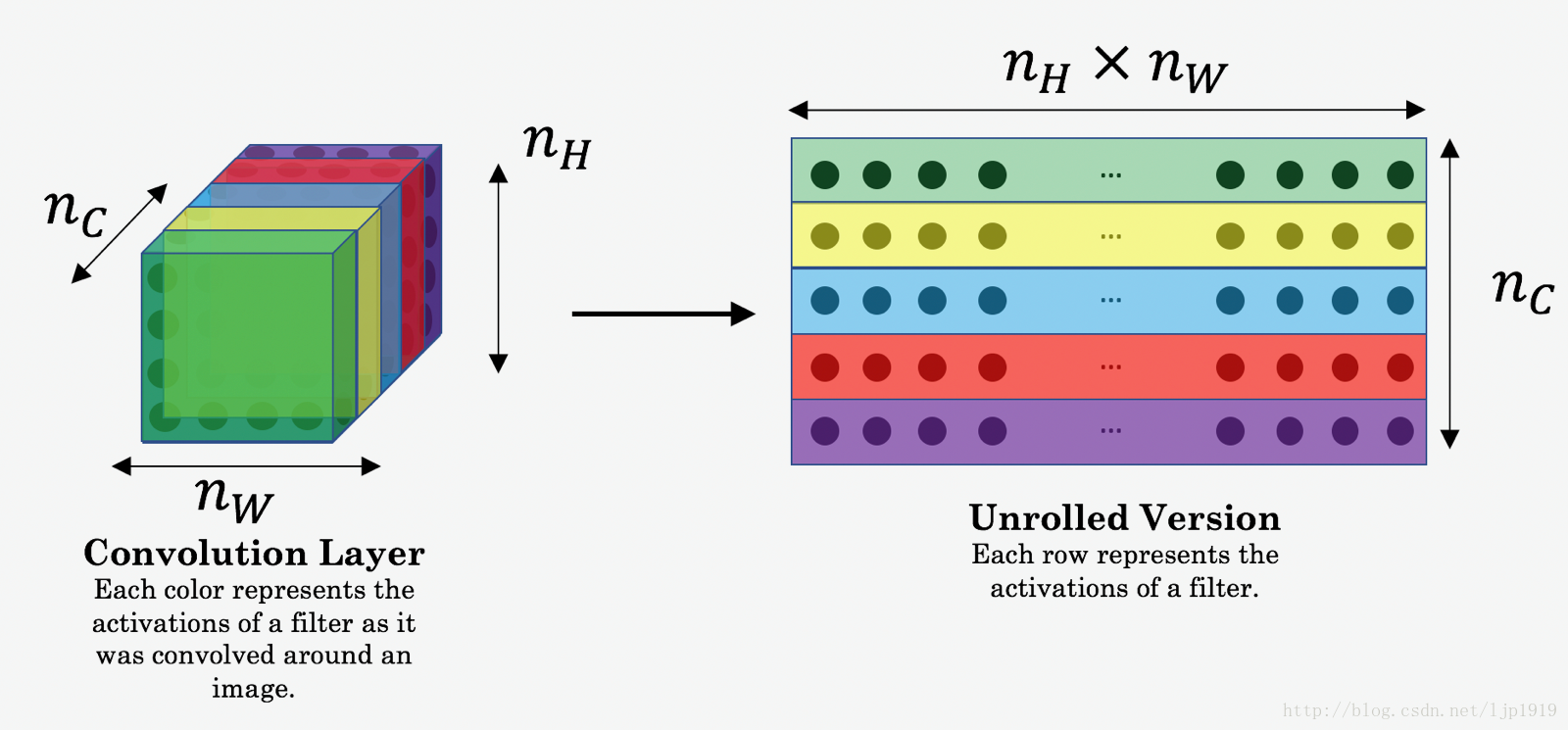
假设我们选取第$l$层的网络进行分析，image C输入到预训练的VGG network，并进行前向传播。 $a^{(C)}$是该层的激活值，其tensor的尺寸= $n_H \times n_W \times n_C$。对于image G做相同的处理：图像 G输入到网络，前向传播。同样记 $a^{(G)}$为对应的激活值。定义content cost function如下：

$$J_{content}(C,G) = \frac{1}{4 \times n_H \times n_W \times n_C}\sum _{ \text{all entries}} (a^{(C)} - a^{(G)})^2\tag{1}$$

这里的 $a^{(C)}$ and $a^{(G)}$ 都是体数据（volumes ），即三维堆叠起来的。 在计算 cost $J_{content}(C,G)$时候，可以展开为2D。其实在计算$J_{content}$, 可以不用，而在计算style 代价函数$J_{style}$时需要。展开方法如下：

content的代价函数实现如下：

# GRADED FUNCTION: compute_content_cost

def compute_content_cost(a_C, a_G):
    """
    Computes the content cost

    Arguments:
    a_C -- tensor of dimension (1, n_H, n_W, n_C), hidden layer activations representing content of the image C 
    a_G -- tensor of dimension (1, n_H, n_W, n_C), hidden layer activations representing content of the image G

    Returns: 
    J_content -- scalar that you compute using equation 1 above.
    """

    ### START CODE HERE ###
    # Retrieve dimensions from a_G (≈1 line)
    m, n_H, n_W, n_C = a_G.get_shape().as_list()

    # Reshape a_C and a_G (≈2 lines)
    a_C_unrolled = tf.transpose(tf.reshape(a_C, [n_H * n_W, n_C]))
    a_G_unrolled = tf.transpose(tf.reshape(a_G, [n_H * n_W, n_C]))

    # compute the cost with tensorflow (≈1 line)
    J_content = tf.reduce_sum(tf.square(tf.subtract(a_C_unrolled,a_G_unrolled)))/(4*n_H*n_W*n_C)
    ### END CODE HERE ###

    return J_content

测试：

tf.reset_default_graph()

with tf.Session() as test:
    tf.set_random_seed(1)
    a_C = tf.random_normal([1, 4, 4, 3], mean=1, stddev=4)
    a_G = tf.random_normal([1, 4, 4, 3], mean=1, stddev=4)
    J_content = compute_content_cost(a_C, a_G)
    print("J_content = " + str(J_content.eval()))

测试结果：

J_content   6.76559 

2-2 Computing the style cost

先看下style图像：

style_image = scipy.misc.imread("images/monet_800600.jpg")
imshow(style_image)

2-2-1 Style matrix

style matrix也称为”Gram matrix.”（格拉姆矩阵） 。在线性代数中，vectors $(v_{1},\dots ,v_{n})$的 Gram matrix G 中各个位置的元素是vector中dot product结果，即${\displaystyle G_{ij} = v_{i}^T v_{j} = np.dot(v_{i}, v_{j}) }$。 $G_{ij}$ 记录的是 $v_i$ 到 $v_j$之间的相似度，如果二者相似度高，则dot product的结果会很大， 即for $G_{ij}$ 值很大。
这里Style matrix (or Gram matrix) 会和generated image $G$可能会在表示上有所冲突，所以具使用的时候，要注意区分。
计算Style matrix，是将unroll结果与unroll的转置相乘：

其结果矩阵尺寸=$(n_C,n_C)$ ，其中$n_C$ 是number of filters。此时的 $G_{ij}$ 度量了activations of filter $i$ 和 activations of filter $j$之间的相似性。Gram的对角线元素，还体现了每个特征在图像中出现的量，例如 $G_{ii}$ 值大，则说明该filter探测到特征在图像中出现频繁。所以，Style matrix $G$ 可以用来度量 image的风格。
代码实现：

# GRADED FUNCTION: gram_matrix

def gram_matrix(A):
    """
    Argument:
    A -- matrix of shape (n_C, n_H*n_W)

    Returns:
    GA -- Gram matrix of A, of shape (n_C, n_C)
    """

    ### START CODE HERE ### (≈1 line)
    GA = tf.matmul(A,tf.transpose(A))
    #tf.matmul是矩阵乘法
    #tf.multiply是点乘，即像素之间的乘法
    ### END CODE HERE ###

    return GA

测试如下：

tf.reset_default_graph()

with tf.Session() as test:
    tf.set_random_seed(1)
    A = tf.random_normal([3, 2*1], mean=1, stddev=4)
    GA = gram_matrix(A)

    print("GA = " + str(GA.eval()))

测试结果：

GA =[[ 6.42230511 -4.42912197 -2.09668207]
[ -4.42912197 19.46583748 19.56387138]
[ -2.09668207 19.56387138 20.6864624 ]] 

2-2-2 Style cost

在计算Style matrix (Gram matrix)后，我们要最小化 “style” image S的Gram matrix和”generated” image G之间的distance。我们先以第$l$层为例，其对应的 style cost定义如下：

$$J_{style}^{[l]}(S,G) = \frac{1}{4 \times {n_C}^2 \times (n_H \times n_W)^2} \sum _{i=1}^{n_C}\sum_{j=1}^{n_C}(G^{(S)}_{ij} - G^{(G)}_{ij})^2\tag{2}$$
$G^{(S)}$ 和 $G^{(G)}$ 分别表示style image和generated image的Gram matrice。
具体的代码实现如下：

# GRADED FUNCTION: compute_layer_style_cost

def compute_layer_style_cost(a_S, a_G):
    """
    Arguments:
    a_S -- tensor of dimension (1, n_H, n_W, n_C), hidden layer activations representing style of the image S 
    a_G -- tensor of dimension (1, n_H, n_W, n_C), hidden layer activations representing style of the image G

    Returns: 
    J_style_layer -- tensor representing a scalar value, style cost defined above by equation (2)
    """

    ### START CODE HERE ###
    # Retrieve dimensions from a_G (≈1 line)
    m, n_H, n_W, n_C = a_G.get_shape().as_list()

    # Reshape the images to have them of shape (n_H*n_W, n_C) (≈2 lines)
    a_S = tf.reshape(a_S, [n_H * n_W, n_C])
    a_G = tf.reshape(a_G, [n_H * n_W, n_C])

    # Computing gram_matrices for both images S and G (≈2 lines)
    GS = gram_matrix(a_S)
    GG = gram_matrix(a_G)

    # Computing the loss (≈1 line)
    J_style_layer = tf.reduce_sum(tf.square(tf.subtract(GS,GG)))/(4*tf.square(tf.to_float(n_C))*tf.square(tf.to_float(n_H*n_W)))
   #J_style_layer = tf.reduce_sum(tf.square(tf.subtract(GS,GG)))/(4 * n_C**2 * (n_W * n_H)**2)

    ### END CODE HERE ###

    return J_style_layer

代码测试如下：

tf.reset_default_graph()

with tf.Session() as test:
    tf.set_random_seed(1)
    a_S = tf.random_normal([1, 4, 4, 3], mean=1, stddev=4)
    a_G = tf.random_normal([1, 4, 4, 3], mean=1, stddev=4)
    J_style_layer = compute_layer_style_cost(a_S, a_G)

    print("J_style_layer = " + str(J_style_layer.eval()))

测试结果输出：

J_style_layer=9.19028

2-2-3 Style Weights

上面，我们仅仅是计算了一层的style cost，我们需要根据不同层的取一定的权重，再将所有层的style cost按照权重进行求和。注：content部分，采用一层是足够的。
实现如下：

def compute_style_cost(model, STYLE_LAYERS):
    """
    Computes the overall style cost from several chosen layers

    Arguments:
    model -- our tensorflow model
    STYLE_LAYERS -- A python list containing:
                        - the names of the layers we would like to extract style from
                        - a coefficient for each of them

    Returns: 
    J_style -- tensor representing a scalar value, style cost defined above by equation (2)
    """

    # initialize the overall style cost
    J_style = 0

    for layer_name, coeff in STYLE_LAYERS:

        # Select the output tensor of the currently selected layer
        out = model[layer_name]

        # Set a_S to be the hidden layer activation from the layer we have selected, by running the session on out
        a_S = sess.run(out)

        # Set a_G to be the hidden layer activation from same layer. Here, a_G references model[layer_name] 
        # and isn't evaluated yet. Later in the code, we'll assign the image G as the model input, so that
        # when we run the session, this will be the activations drawn from the appropriate layer, with G as input.
        a_G = out

        # Compute style_cost for the current layer
        J_style_layer = compute_layer_style_cost(a_S, a_G)

        # Add coeff * J_style_layer of this layer to overall style cost
        J_style += coeff * J_style_layer

    return J_style

2-3 total cost to optimize

总的代价函数定义如下：

$$J(G) = \alpha J_{content}(C,G) + \beta J_{style}(S,G)$$
函数实现：

# GRADED FUNCTION: total_cost

def total_cost(J_content, J_style, alpha = 10, beta = 40):
    """
    Computes the total cost function

    Arguments:
    J_content -- content cost coded above
    J_style -- style cost coded above
    alpha -- hyperparameter weighting the importance of the content cost
    beta -- hyperparameter weighting the importance of the style cost

    Returns:
    J -- total cost as defined by the formula above.
    """

    ### START CODE HERE ### (≈1 line)
    J = alpha*J_content+beta*J_style
    ### END CODE HERE ###

    return J

函数测试：

tf.reset_default_graph()

with tf.Session() as test:
    np.random.seed(3)
    J_content = np.random.randn()    
    J_style = np.random.randn()
    J = total_cost(J_content, J_style)
    print("J = " + str(J))

测试结果：

J=35.34667875478276 

3- 优化

Neural Style Transfer的实现步骤如下：

1. Create an Interactive Session
2. Load the content image
3. Load the style image
4. Randomly initialize the image to be generated
5. Load the VGG16 model
6. Build the TensorFlow graph:
   
   • Run the content image through the VGG16 model and compute the content cost
   • Run the style image through the VGG16 model and compute the style cost
   • Compute the total cost
   • Define the optimizer and the learning rate
7. Initialize the TensorFlow graph and run it for a large number of iterations, updating the generated image at every step.

各步骤的具体细节如下：

# Reset the graph
tf.reset_default_graph()

# Start interactive session
sess = tf.InteractiveSession()

加载 “content” image并进行 reshape, and normalize：

content_image = scipy.misc.imread("images/louvre_small.jpg")
content_image = reshape_and_normalize_image(content_image)

加载 “style” image并进行 reshape, and normalize：

style_image = scipy.misc.imread("images/monet.jpg")
style_image = reshape_and_normalize_image(style_image)

“generated” image初始化： 通过对content_image添加噪声完成。添加的噪声较大，但是依然能够使其与content_image有一些些的相关性。这有助于”generated” image 能够更快速地与”content” image相匹配。

generated_image = generate_noise_image(content_image)
imshow(generated_image[0])

加载VGG-16模型：

model = load_vgg_model("pretrained-model/imagenet-vgg-verydeep-19.mat")

为了计算 content cost，我们需要将a_C and a_G 输入到合适的隐藏层，这里我们采用是 conv4_2层：

1. 将content image输入到VGG model.
2. Set a_C to be the tensor giving the hidden layer activation for layer “conv4_2”.
3. Set a_G to be the tensor giving the hidden layer activation for the same layer.
4. Compute the content cost using a_C and a_G.

实现如下：

# Assign the content image to be the input of the VGG model.  
sess.run(model['input'].assign(content_image))

# Select the output tensor of layer conv4_2
out = model['conv4_2']

# Set a_C to be the hidden layer activation from the layer we have selected
a_C = sess.run(out)

# Set a_G to be the hidden layer activation from same layer. Here, a_G references model['conv4_2'] 
# and isn't evaluated yet. Later in the code, we'll assign the image G as the model input, so that
# when we run the session, this will be the activations drawn from the appropriate layer, with G as input.
a_G = out#a_G is a tensor and hasn't been evaluated


# Compute the content cost
J_content = compute_content_cost(a_C, a_G)

注意：上面的a_G 还未被估计，其更新是在每轮迭代之后。
对于 “style” image ：

# Assign the input of the model to be the "style" image 
sess.run(model['input'].assign(style_image))

# Compute the style cost
J_style = compute_style_cost(model, STYLE_LAYERS)

计算整体代价：

### START CODE HERE ### (1 line)
J = total_cost(J_content, J_style, alpha = 10, beta = 40)
### END CODE HERE ###

优化：

# define optimizer (1 line)
optimizer = tf.train.AdamOptimizer(2.0)

# define train_step (1 line)
train_step = optimizer.minimize(J)

完整的模型实现：

def model_nn(sess, input_image, num_iterations = 200):

    # Initialize global variables (you need to run the session on the initializer)
    ### START CODE HERE ### (1 line)
    sess.run(tf.global_variables_initializer())
    ### END CODE HERE ###

    # Run the noisy input image (initial generated image) through the model. Use assign().
    ### START CODE HERE ### (1 line)
    generated_image = sess.run(model['input'].assign(input_image))
    ### END CODE HERE ###

    for i in range(num_iterations):

        # Run the session on the train_step to minimize the total cost
        ### START CODE HERE ### (1 line)
        sess.run(train_step)
        ### END CODE HERE ###

        # Compute the generated image by running the session on the current model['input']
        ### START CODE HERE ### (1 line)
        generated_image = sess.run(model['input'])
        ### END CODE HERE ###

        # Print every 20 iteration.
        if i%20 == 0:
            Jt, Jc, Js = sess.run([J, J_content, J_style])
            print("Iteration " + str(i) + " :")
            print("total cost = " + str(Jt))
            print("content cost = " + str(Jc))
            print("style cost = " + str(Js))

            # save current generated image in the "/output" directory
            save_image("output/" + str(i) + ".png", generated_image)

    # save last generated image
    save_image('output/generated_image.jpg', generated_image)

    return generated_image

模型测试：

model_nn(sess, generated_image)

结果展示如下：
content图：

style图：

生成的图：

4- 其他图像的测试：

重新输入content image和style image：

content_image = scipy.misc.imread("images/my_content.jpg")
style_image = scipy.misc.imread("images/my_style.jpg")

我们需要调整的超参数：

• Which layers are responsible for representing the style? STYLE_LAYERS
• 迭代次数， num_iterations
• What is the relative weighting between content and style? alpha/beta