Neural Networks and Deep Learning CH1

CHAPTER 1
Using neural nets to recognize handwritten digits

这一章主要介绍并构建了一个朴素的神经网络来实现准确率在96%左右的手写识别。

Perceptrons

这一节首先介绍了感知机(Perceptrons)，虽然现在常用的激活函数是Sigomid，在NTU课程中还学到了RELU，但如书中所说，了解Perceptrons能让我们更了解其他激活函数是如何定义的。

感知机的工作原理很简单：

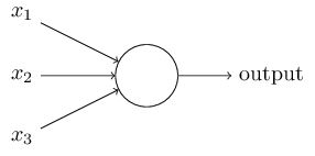
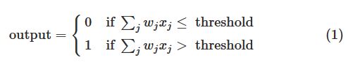
将输入与边权的乘积和与threshold相比较输入01即可。

如果令$b = -threshold$，则有：

感知机的实际意义是可以做一些带权重的决断，更进一步，他可以模拟各种逻辑计算。

这里我开了一个脑洞，游戏《minecraft》中，可以用红石来模拟各种逻辑电路，于是有人基于此做出了游戏中的计算机。这么一想，我感觉最简单的感知机就已经超越了硬件方面的逻辑电路设计。延伸开来，未来的神经网络会不会替代目前硬件的电路设计？

Sigmoid neurons

这一节我觉得重点在于引入了如何训练神经网络的方向：
如果对于一个权重，其微小的改变能在output中体现出来，那么对于神经网络的训练就有方向可以进行。

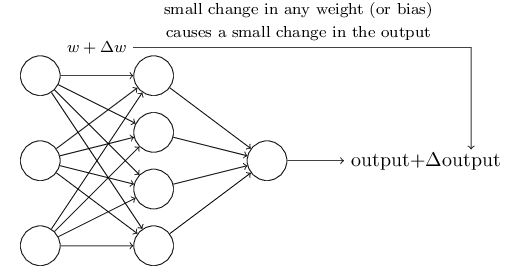
而此时如果神经网络使用的激活函数为perceptrons，那么这种改变将不会在output中体现出来。实际上，在权重上一点微小的改变有时会导致output的结果完全翻转（0-1，1-0）。

也正因如此才提出了sigmoid神经元。sigmoid神经元和perceptrons很像，改进的是权重的改变能够在output中体现出来。

sigmoid函数已经很熟悉了：$σ(z)≡\frac{1}{1+e^{−z}}$。
output如何改变也有公式可以计算：

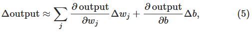
这个公式告诉我们output的变化是权重和偏差变化的线性函数，因此可以很简单的衡量其间的关系。

The architecture of neural networks

对于神经网络已经很熟悉了。

这一节中提到了RNN。之前并不觉得RNN很厉害，后来看了老师的分享和一些资料，了解了原来LSTM是目前最接近人脑思考方式的神经网络。

A simple network to classify handwritten digits

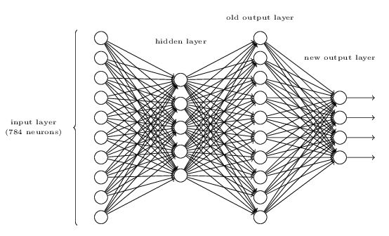
这一节提出了一个解决28*28像素点手写图像识别的神经网络。
我觉得有启发性的是最后提出来只用4位2进制的输出来表示十个数字：

可惜的是很难直接用3层来实现它，书中给出的原因是二进制位和手写数字的特征很难有逻辑上的对应关系。

Learning with gradient descent

这一节详细地介绍了gradient descent的来龙去脉。

首先是cost function的定义：

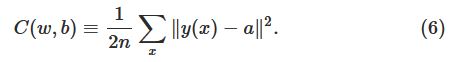
其中$w,b$是参数，$a$是输入为$x$时的输出向量。我们的目标是找到$w,b$使得cost function越小越好。

假设有两个参数$v_1,v_2$，而我们让一个小球在$v_1$方向移动$Δv_1$，在$v_2$方向移动$Δv_2$，则$C$的变化为：

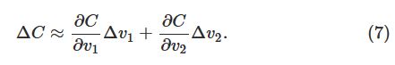
我们要找到一种选择$Δv_1，Δv_2$的方法使得$ΔC$为负数。为此，定义：
$Δv≡(Δv_1,Δv_2)^T$

$∇C≡(\frac{∂C}{∂v_1},\frac{∂C}{∂v_2})^T$。

因此：

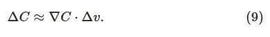
注意三角形的朝向。

由上，可以有一种使得$ΔC$为负的方式，其中$\eta$为学习率：

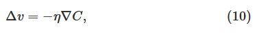
因为：

因此可以得到一种更新参数 v <script id="MathJax-Element-19" type="math/tex">v</script>的方式：

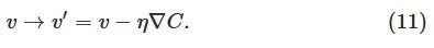
从二维拓展到多维也是如此更新。

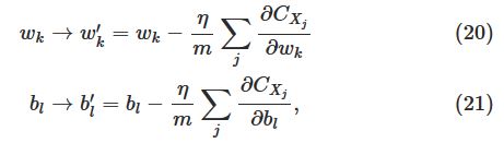
回到神经网络的训练，其更新方法为：

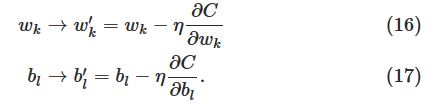
stochastic gradient descent的更新方法为：

Implementing our network to classify digits

这一节用python定义了朴素版本的神经网络来进行手写数字识别。用的是stochastic gradient descent（SGD）。没有详细解释的backpropation会在下一章讨论。

书中的代码可以改进的地方挺多的，首先是之后章节会提出的优化，这里不说了。
其次是，代码中的for循环完全可以使用矩阵运算替代。
从中学到一点是xrange的使用，在大量使用循环时，xrange比range更省时间和空间。具体原因是xrange不会把枚举的数生成list而range会。

代码：

"""
network.py
~~~~~~~~~~

A module to implement the stochastic gradient descent learning
algorithm for a feedforward neural network.  Gradients are calculated
using backpropagation.  Note that I have focused on making the code
simple, easily readable, and easily modifiable.  It is not optimized,
and omits many desirable features.
"""

#### Libraries
# Standard library
import random

# Third-party libraries
import numpy as np

class Network(object):

    def __init__(self, sizes):
        """The list ``sizes`` contains the number of neurons in the
        respective layers of the network.  For example, if the list
        was [2, 3, 1] then it would be a three-layer network, with the
        first layer containing 2 neurons, the second layer 3 neurons,
        and the third layer 1 neuron.  The biases and weights for the
        network are initialized randomly, using a Gaussian
        distribution with mean 0, and variance 1.  Note that the first
        layer is assumed to be an input layer, and by convention we
        won't set any biases for those neurons, since biases are only
        ever used in computing the outputs from later layers."""
        self.num_layers = len(sizes)
        self.sizes = sizes
        self.biases = [np.random.randn(y, 1) for y in sizes[1:]]
        self.weights = [np.random.randn(y, x)
                        for x, y in zip(sizes[:-1], sizes[1:])]

    def feedforward(self, a):
        """Return the output of the network if ``a`` is input."""
        for b, w in zip(self.biases, self.weights):
            a = sigmoid(np.dot(w, a)+b)
        return a

    def SGD(self, training_data, epochs, mini_batch_size, eta,
            test_data=None):
        """Train the neural network using mini-batch stochastic
        gradient descent.  The ``training_data`` is a list of tuples
        ``(x, y)`` representing the training inputs and the desired
        outputs.  The other non-optional parameters are
        self-explanatory.  If ``test_data`` is provided then the
        network will be evaluated against the test data after each
        epoch, and partial progress printed out.  This is useful for
        tracking progress, but slows things down substantially."""
        if test_data: n_test = len(test_data)
        n = len(training_data)
        for j in xrange(epochs):
            random.shuffle(training_data)
            mini_batches = [
                training_data[k:k+mini_batch_size]
                for k in xrange(0, n, mini_batch_size)]
            for mini_batch in mini_batches:
                self.update_mini_batch(mini_batch, eta)
            if test_data:
                print "Epoch {0}: {1} / {2}".format(
                    j, self.evaluate(test_data), n_test)
            else:
                print "Epoch {0} complete".format(j)

    def update_mini_batch(self, mini_batch, eta):
        """Update the network's weights and biases by applying
        gradient descent using backpropagation to a single mini batch.
        The ``mini_batch`` is a list of tuples ``(x, y)``, and ``eta``
        is the learning rate."""
        nabla_b = [np.zeros(b.shape) for b in self.biases]
        nabla_w = [np.zeros(w.shape) for w in self.weights]
        for x, y in mini_batch:
            delta_nabla_b, delta_nabla_w = self.backprop(x, y)
            nabla_b = [nb+dnb for nb, dnb in zip(nabla_b, delta_nabla_b)]
            nabla_w = [nw+dnw for nw, dnw in zip(nabla_w, delta_nabla_w)]
        self.weights = [w-(eta/len(mini_batch))*nw
                        for w, nw in zip(self.weights, nabla_w)]
        self.biases = [b-(eta/len(mini_batch))*nb
                       for b, nb in zip(self.biases, nabla_b)]

    def backprop(self, x, y):
        """Return a tuple ``(nabla_b, nabla_w)`` representing the
        gradient for the cost function C_x.  ``nabla_b`` and
        ``nabla_w`` are layer-by-layer lists of numpy arrays, similar
        to ``self.biases`` and ``self.weights``."""
        nabla_b = [np.zeros(b.shape) for b in self.biases]
        nabla_w = [np.zeros(w.shape) for w in self.weights]
        # feedforward
        activation = x
        activations = [x] # list to store all the activations, layer by layer
        zs = [] # list to store all the z vectors, layer by layer
        for b, w in zip(self.biases, self.weights):
            z = np.dot(w, activation)+b
            zs.append(z)
            activation = sigmoid(z)
            activations.append(activation)
        # backward pass
        delta = self.cost_derivative(activations[-1], y) * \
            sigmoid_prime(zs[-1])
        nabla_b[-1] = delta
        nabla_w[-1] = np.dot(delta, activations[-2].transpose())
        # Note that the variable l in the loop below is used a little
        # differently to the notation in Chapter 2 of the book.  Here,
        # l = 1 means the last layer of neurons, l = 2 is the
        # second-last layer, and so on.  It's a renumbering of the
        # scheme in the book, used here to take advantage of the fact
        # that Python can use negative indices in lists.
        for l in xrange(2, self.num_layers):
            z = zs[-l]
            sp = sigmoid_prime(z)
            delta = np.dot(self.weights[-l+1].transpose(), delta) * sp
            nabla_b[-l] = delta
            nabla_w[-l] = np.dot(delta, activations[-l-1].transpose())
        return (nabla_b, nabla_w)

    def evaluate(self, test_data):
        """Return the number of test inputs for which the neural
        network outputs the correct result. Note that the neural
        network's output is assumed to be the index of whichever
        neuron in the final layer has the highest activation."""
        test_results = [(np.argmax(self.feedforward(x)), y)
                        for (x, y) in test_data]
        return sum(int(x == y) for (x, y) in test_results)

    def cost_derivative(self, output_activations, y):
        """Return the vector of partial derivatives \partial C_x /
        \partial a for the output activations."""
        return (output_activations-y)

#### Miscellaneous functions
def sigmoid(z):
    """The sigmoid function."""
    return 1.0/(1.0+np.exp(-z))

def sigmoid_prime(z):
    """Derivative of the sigmoid function."""
    return sigmoid(z)*(1-sigmoid(z))

这里还做了几个实验，横向比较了学习率对结果的影响；纵向比较了随机猜测，黑色占比猜测，svm的正确率。

数据的读取：

"""
mnist_loader
~~~~~~~~~~~~

A library to load the MNIST image data.  For details of the data
structures that are returned, see the doc strings for ``load_data``
and ``load_data_wrapper``.  In practice, ``load_data_wrapper`` is the
function usually called by our neural network code.
"""

#### Libraries
# Standard library
import cPickle
import gzip

# Third-party libraries
import numpy as np

def load_data():
    """Return the MNIST data as a tuple containing the training data,
    the validation data, and the test data.

    The ``training_data`` is returned as a tuple with two entries.
    The first entry contains the actual training images.  This is a
    numpy ndarray with 50,000 entries.  Each entry is, in turn, a
    numpy ndarray with 784 values, representing the 28 * 28 = 784
    pixels in a single MNIST image.

    The second entry in the ``training_data`` tuple is a numpy ndarray
    containing 50,000 entries.  Those entries are just the digit
    values (0...9) for the corresponding images contained in the first
    entry of the tuple.

    The ``validation_data`` and ``test_data`` are similar, except
    each contains only 10,000 images.

    This is a nice data format, but for use in neural networks it's
    helpful to modify the format of the ``training_data`` a little.
    That's done in the wrapper function ``load_data_wrapper()``, see
    below.
    """
    f = gzip.open('../data/mnist.pkl.gz', 'rb')
    training_data, validation_data, test_data = cPickle.load(f)
    f.close()
    return (training_data, validation_data, test_data)

def load_data_wrapper():
    """Return a tuple containing ``(training_data, validation_data,
    test_data)``. Based on ``load_data``, but the format is more
    convenient for use in our implementation of neural networks.

    In particular, ``training_data`` is a list containing 50,000
    2-tuples ``(x, y)``.  ``x`` is a 784-dimensional numpy.ndarray
    containing the input image.  ``y`` is a 10-dimensional
    numpy.ndarray representing the unit vector corresponding to the
    correct digit for ``x``.

    ``validation_data`` and ``test_data`` are lists containing 10,000
    2-tuples ``(x, y)``.  In each case, ``x`` is a 784-dimensional
    numpy.ndarry containing the input image, and ``y`` is the
    corresponding classification, i.e., the digit values (integers)
    corresponding to ``x``.

    Obviously, this means we're using slightly different formats for
    the training data and the validation / test data.  These formats
    turn out to be the most convenient for use in our neural network
    code."""
    tr_d, va_d, te_d = load_data()
    training_inputs = [np.reshape(x, (784, 1)) for x in tr_d[0]]
    training_results = [vectorized_result(y) for y in tr_d[1]]
    training_data = zip(training_inputs, training_results)
    validation_inputs = [np.reshape(x, (784, 1)) for x in va_d[0]]
    validation_data = zip(validation_inputs, va_d[1])
    test_inputs = [np.reshape(x, (784, 1)) for x in te_d[0]]
    test_data = zip(test_inputs, te_d[1])
    return (training_data, validation_data, test_data)

def vectorized_result(j):
    """Return a 10-dimensional unit vector with a 1.0 in the jth
    position and zeroes elsewhere.  This is used to convert a digit
    (0...9) into a corresponding desired output from the neural
    network."""
    e = np.zeros((10, 1))
    e[j] = 1.0
    return e

电子书URL:http://neuralnetworksanddeeplearning.com/chap1.html#the_architecture_of_neural_networks