Tensorflow一些常用基本概念与函数

原文地址：http://blog.csdn.net/lenbow/article/details/52152766

1、tensorflow的基本运作

为了快速的熟悉TensorFlow编程，下面从一段简单的代码开始：

import tensorflow as tf
 #定义‘符号’变量，也称为占位符
 a = tf.placeholder("float")
 b = tf.placeholder("float")

 y = tf.mul(a, b) #构造一个op节点

 sess = tf.Session()#建立会话
 #运行会话，输入数据，并计算节点，同时打印结果
 print sess.run(y, feed_dict={a: 3, b: 3})
 # 任务完成, 关闭会话.
 sess.close()
 
 
1
2
3
4
5
6
7
8
9
10
11
12
 
 
1
2
3
4
5
6
7
8
9
10
11
12

其中tf.mul(a, b)函数便是tf的一个基本的算数运算，接下来介绍跟多的相关函数。

2、tf函数

TensorFlow 将图形定义转换成分布式执行的操作, 以充分利用可用的计算资源(如 CPU 或 GPU。一般你不需要显式指定使用 CPU 还是 GPU, TensorFlow 能自动检测。如果检测到 GPU, TensorFlow 会尽可能地利用找到的第一个 GPU 来执行操作.
并行计算能让代价大的算法计算加速执行，TensorFlow也在实现上对复杂操作进行了有效的改进。大部分核相关的操作都是设备相关的实现，比如GPU。下面是一些重要的操作/核：

操作组	操作
Maths	Add, Sub, Mul, Div, Exp, Log, Greater, Less, Equal
Array	Concat, Slice, Split, Constant, Rank, Shape, Shuffle
Matrix	MatMul, MatrixInverse, MatrixDeterminant
Neuronal Network	SoftMax, Sigmoid, ReLU, Convolution2D, MaxPool
Checkpointing	Save, Restore
Queues and syncronizations	Enqueue, Dequeue, MutexAcquire, MutexRelease
Flow control	Merge, Switch, Enter, Leave, NextIteration

TensorFlow的算术操作如下：

操作	描述
tf.add(x, y, name=None)	求和
tf.sub(x, y, name=None)	减法
tf.mul(x, y, name=None)	乘法
tf.div(x, y, name=None)	除法
tf.mod(x, y, name=None)	取模
tf.abs(x, name=None)	求绝对值
tf.neg(x, name=None)	取负 (y = -x).
tf.sign(x, name=None)	返回符号 y = sign(x) = -1 if x < 0; 0 if x == 0; 1 if x > 0.
tf.inv(x, name=None)	取反
tf.square(x, name=None)	计算平方 (y = x * x = x^2).
tf.round(x, name=None)	舍入最接近的整数 # ‘a’ is [0.9, 2.5, 2.3, -4.4] tf.round(a) ==> [ 1.0, 3.0, 2.0, -4.0 ]
tf.sqrt(x, name=None)	开根号 (y = \sqrt{x} = x^{1/2}).
tf.pow(x, y, name=None)	幂次方  # tensor ‘x’ is [[2, 2], [3, 3]] # tensor ‘y’ is [[8, 16], [2, 3]] tf.pow(x, y) ==> [[256, 65536], [9, 27]]
tf.exp(x, name=None)	计算e的次方
tf.log(x, name=None)	计算log，一个输入计算e的ln，两输入以第二输入为底
tf.maximum(x, y, name=None)	返回最大值 (x > y ? x : y)
tf.minimum(x, y, name=None)	返回最小值 (x < y ? x : y)
tf.cos(x, name=None)	三角函数cosine
tf.sin(x, name=None)	三角函数sine
tf.tan(x, name=None)	三角函数tan
tf.atan(x, name=None)	三角函数ctan

---

张量操作Tensor Transformations

• 数据类型转换Casting

操作	描述
tf.string_to_number (string_tensor, out_type=None, name=None)	字符串转为数字
tf.to_double(x, name=’ToDouble’)	转为64位浮点类型–float64
tf.to_float(x, name=’ToFloat’)	转为32位浮点类型–float32
tf.to_int32(x, name=’ToInt32’)	转为32位整型–int32
tf.to_int64(x, name=’ToInt64’)	转为64位整型–int64
tf.cast(x, dtype, name=None)	将x或者x.values转换为dtype # tensor a is [1.8, 2.2], dtype=tf.float tf.cast(a, tf.int32) ==> [1, 2] # dtype=tf.int32

• 形状操作Shapes and Shaping

操作	描述
tf.shape(input, name=None)	返回数据的shape # ‘t’ is [[[1, 1, 1], [2, 2, 2]], [[3, 3, 3], [4, 4, 4]]] shape(t) ==> [2, 2, 3]
tf.size(input, name=None)	返回数据的元素数量 # ‘t’ is [[[1, 1, 1], [2, 2, 2]], [[3, 3, 3], [4, 4, 4]]]] size(t) ==> 12
tf.rank(input, name=None)	返回tensor的rank 注意：此rank不同于矩阵的rank， tensor的rank表示一个tensor需要的索引数目来唯一表示任何一个元素 也就是通常所说的 “order”, “degree”或”ndims” #’t’ is [[[1, 1, 1], [2, 2, 2]], [[3, 3, 3], [4, 4, 4]]] # shape of tensor ‘t’ is [2, 2, 3] rank(t) ==> 3
tf.reshape(tensor, shape, name=None)	改变tensor的形状 # tensor ‘t’ is [1, 2, 3, 4, 5, 6, 7, 8, 9] # tensor ‘t’ has shape [9] reshape(t, [3, 3]) ==>  [[1, 2, 3], [4, 5, 6], [7, 8, 9]] #如果shape有元素[-1],表示在该维度打平至一维 # -1 将自动推导得为 9: reshape(t, [2, -1]) ==>  [[1, 1, 1, 2, 2, 2, 3, 3, 3], [4, 4, 4, 5, 5, 5, 6, 6, 6]]
tf.expand_dims(input, dim, name=None)	插入维度1进入一个tensor中 #该操作要求-1-input.dims() # ‘t’ is a tensor of shape [2] shape(expand_dims(t, 0)) ==> [1, 2] shape(expand_dims(t, 1)) ==> [2, 1] shape(expand_dims(t, -1)) ==> [2, 1] <= dim <= input.dims()

• 切片与合并（Slicing and Joining）

操作	描述
tf.slice(input_, begin, size, name=None)	对tensor进行切片操作 其中size[i] = input.dim_size(i) - begin[i] 该操作要求 0 <= begin[i] <= begin[i] + size[i] <= Di for i in [0, n] #’input’ is  #[[[1, 1, 1], [2, 2, 2]],[[3, 3, 3], [4, 4, 4]],[[5, 5, 5], [6, 6, 6]]] tf.slice(input, [1, 0, 0], [1, 1, 3]) ==> [[[3, 3, 3]]] tf.slice(input, [1, 0, 0], [1, 2, 3]) ==>  [[[3, 3, 3], [4, 4, 4]]] tf.slice(input, [1, 0, 0], [2, 1, 3]) ==>  [[[3, 3, 3]], [[5, 5, 5]]]
tf.split(split_dim, num_split, value, name=’split’)	沿着某一维度将tensor分离为num_split tensors # ‘value’ is a tensor with shape [5, 30] # Split ‘value’ into 3 tensors along dimension 1 split0, split1, split2 = tf.split(1, 3, value) tf.shape(split0) ==> [5, 10]
tf.concat(concat_dim, values, name=’concat’)	沿着某一维度连结tensor t1 = [[1, 2, 3], [4, 5, 6]] t2 = [[7, 8, 9], [10, 11, 12]] tf.concat(0, [t1, t2]) ==> [[1, 2, 3], [4, 5, 6], [7, 8, 9], [10, 11, 12]] tf.concat(1, [t1, t2]) ==> [[1, 2, 3, 7, 8, 9], [4, 5, 6, 10, 11, 12]] 如果想沿着tensor一新轴连结打包,那么可以： tf.concat(axis, [tf.expand_dims(t, axis) for t in tensors]) 等同于tf.pack(tensors, axis=axis)
tf.pack(values, axis=0, name=’pack’)	将一系列rank-R的tensor打包为一个rank-(R+1)的tensor # ‘x’ is [1, 4], ‘y’ is [2, 5], ‘z’ is [3, 6] pack([x, y, z]) => [[1, 4], [2, 5], [3, 6]]  # 沿着第一维pack pack([x, y, z], axis=1) => [[1, 2, 3], [4, 5, 6]] 等价于tf.pack([x, y, z]) = np.asarray([x, y, z])
tf.reverse(tensor, dims, name=None)	沿着某维度进行序列反转 其中dim为列表，元素为bool型，size等于rank(tensor) # tensor ‘t’ is  [[[[ 0, 1, 2, 3], #[ 4, 5, 6, 7], #[ 8, 9, 10, 11]], #[[12, 13, 14, 15], #[16, 17, 18, 19], #[20, 21, 22, 23]]]] # tensor ‘t’ shape is [1, 2, 3, 4] # ‘dims’ is [False, False, False, True] reverse(t, dims) ==> [[[[ 3, 2, 1, 0], [ 7, 6, 5, 4], [ 11, 10, 9, 8]], [[15, 14, 13, 12], [19, 18, 17, 16], [23, 22, 21, 20]]]]
tf.transpose(a, perm=None, name=’transpose’)	调换tensor的维度顺序 按照列表perm的维度排列调换tensor顺序， 如为定义，则perm为(n-1…0) # ‘x’ is [[1 2 3],[4 5 6]] tf.transpose(x) ==> [[1 4], [2 5],[3 6]] # Equivalently tf.transpose(x, perm=[1, 0]) ==> [[1 4],[2 5], [3 6]]
tf.gather(params, indices, validate_indices=None, name=None)	合并索引indices所指示params中的切片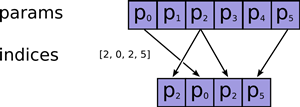
tf.one_hot (indices, depth, on_value=None, off_value=None, axis=None, dtype=None, name=None)	indices = [0, 2, -1, 1] depth = 3 on_value = 5.0  off_value = 0.0  axis = -1  #Then output is [4 x 3]:  output =  [5.0 0.0 0.0] // one_hot(0)  [0.0 0.0 5.0] // one_hot(2)  [0.0 0.0 0.0] // one_hot(-1)  [0.0 5.0 0.0] // one_hot(1)

---

矩阵相关运算

操作	描述
tf.diag(diagonal, name=None)	返回一个给定对角值的对角tensor # ‘diagonal’ is [1, 2, 3, 4] tf.diag(diagonal) ==>  [[1, 0, 0, 0] [0, 2, 0, 0] [0, 0, 3, 0] [0, 0, 0, 4]]
tf.diag_part(input, name=None)	功能与上面相反
tf.trace(x, name=None)	求一个2维tensor足迹，即对角值diagonal之和
tf.transpose(a, perm=None, name=’transpose’)	调换tensor的维度顺序 按照列表perm的维度排列调换tensor顺序， 如为定义，则perm为(n-1…0) # ‘x’ is [[1 2 3],[4 5 6]] tf.transpose(x) ==> [[1 4], [2 5],[3 6]] # Equivalently tf.transpose(x, perm=[1, 0]) ==> [[1 4],[2 5], [3 6]]
tf.matmul(a, b, transpose_a=False,  transpose_b=False, a_is_sparse=False,  b_is_sparse=False, name=None)	矩阵相乘
tf.matrix_determinant(input, name=None)	返回方阵的行列式
tf.matrix_inverse(input, adjoint=None, name=None)	求方阵的逆矩阵，adjoint为True时，计算输入共轭矩阵的逆矩阵
tf.cholesky(input, name=None)	对输入方阵cholesky分解， 即把一个对称正定的矩阵表示成一个下三角矩阵L和其转置的乘积的分解A=LL^T
tf.matrix_solve(matrix, rhs, adjoint=None, name=None)	求解tf.matrix_solve(matrix, rhs, adjoint=None, name=None) matrix为方阵shape为[M,M],rhs的shape为[M,K]，output为[M,K]

---

复数操作

操作	描述
tf.complex(real, imag, name=None)	将两实数转换为复数形式 # tensor ‘real’ is [2.25, 3.25] # tensor imag is [4.75, 5.75] tf.complex(real, imag) ==> [[2.25 + 4.75j], [3.25 + 5.75j]]
tf.complex_abs(x, name=None)	计算复数的绝对值，即长度。 # tensor ‘x’ is [[-2.25 + 4.75j], [-3.25 + 5.75j]] tf.complex_abs(x) ==> [5.25594902, 6.60492229]
tf.conj(input, name=None)	计算共轭复数
tf.imag(input, name=None) tf.real(input, name=None)	提取复数的虚部和实部
tf.fft(input, name=None)	计算一维的离散傅里叶变换，输入数据类型为complex64

---

归约计算(Reduction)

操作	描述
tf.reduce_sum(input_tensor, reduction_indices=None,  keep_dims=False, name=None)	计算输入tensor元素的和，或者安照reduction_indices指定的轴进行求和 # ‘x’ is [[1, 1, 1] # [1, 1, 1]] tf.reduce_sum(x) ==> 6 tf.reduce_sum(x, 0) ==> [2, 2, 2] tf.reduce_sum(x, 1) ==> [3, 3] tf.reduce_sum(x, 1, keep_dims=True) ==> [[3], [3]] tf.reduce_sum(x, [0, 1]) ==> 6
tf.reduce_prod(input_tensor,  reduction_indices=None,  keep_dims=False, name=None)	计算输入tensor元素的乘积，或者安照reduction_indices指定的轴进行求乘积
tf.reduce_min(input_tensor,  reduction_indices=None,  keep_dims=False, name=None)	求tensor中最小值
tf.reduce_max(input_tensor,  reduction_indices=None,  keep_dims=False, name=None)	求tensor中最大值
tf.reduce_mean(input_tensor,  reduction_indices=None,  keep_dims=False, name=None)	求tensor中平均值
tf.reduce_all(input_tensor,  reduction_indices=None,  keep_dims=False, name=None)	对tensor中各个元素求逻辑’与’ # ‘x’ is  # [[True, True] # [False, False]] tf.reduce_all(x) ==> False tf.reduce_all(x, 0) ==> [False, False] tf.reduce_all(x, 1) ==> [True, False]
tf.reduce_any(input_tensor,  reduction_indices=None,  keep_dims=False, name=None)	对tensor中各个元素求逻辑’或’
tf.accumulate_n(inputs, shape=None,  tensor_dtype=None, name=None)	计算一系列tensor的和 # tensor ‘a’ is [[1, 2], [3, 4]] # tensor b is [[5, 0], [0, 6]] tf.accumulate_n([a, b, a]) ==> [[7, 4], [6, 14]]
tf.cumsum(x, axis=0, exclusive=False,  reverse=False, name=None)	求累积和 tf.cumsum([a, b, c]) ==> [a, a + b, a + b + c] tf.cumsum([a, b, c], exclusive=True) ==> [0, a, a + b] tf.cumsum([a, b, c], reverse=True) ==> [a + b + c, b + c, c] tf.cumsum([a, b, c], exclusive=True, reverse=True) ==> [b + c, c, 0]

---

分割(Segmentation)

操作	描述
tf.segment_sum(data, segment_ids, name=None)	根据segment_ids的分段计算各个片段的和 其中segment_ids为一个size与data第一维相同的tensor 其中id为int型数据，最大id不大于size c = tf.constant([[1,2,3,4], [-1,-2,-3,-4], [5,6,7,8]]) tf.segment_sum(c, tf.constant([0, 0, 1])) ==>[[0 0 0 0]  [5 6 7 8]] 上面例子分为[0,1]两id,对相同id的data相应数据进行求和, 并放入结果的相应id中， 且segment_ids只升不降
tf.segment_prod(data, segment_ids, name=None)	根据segment_ids的分段计算各个片段的积
tf.segment_min(data, segment_ids, name=None)	根据segment_ids的分段计算各个片段的最小值
tf.segment_max(data, segment_ids, name=None)	根据segment_ids的分段计算各个片段的最大值
tf.segment_mean(data, segment_ids, name=None)	根据segment_ids的分段计算各个片段的平均值
tf.unsorted_segment_sum(data, segment_ids, num_segments, name=None)	与tf.segment_sum函数类似， 不同在于segment_ids中id顺序可以是无序的
tf.sparse_segment_sum(data, indices,  segment_ids, name=None)	输入进行稀疏分割求和 c = tf.constant([[1,2,3,4], [-1,-2,-3,-4], [5,6,7,8]]) # Select two rows, one segment. tf.sparse_segment_sum(c, tf.constant([0, 1]), tf.constant([0, 0]))  ==> [[0 0 0 0]] 对原data的indices为[0,1]位置的进行分割， 并按照segment_ids的分组进行求和

---

序列比较与索引提取(Sequence Comparison and Indexing)

操作	描述
tf.argmin(input, dimension, name=None)	返回input最小值的索引index
tf.argmax(input, dimension, name=None)	返回input最大值的索引index
tf.listdiff(x, y, name=None)	返回x，y中不同值的索引
tf.where(input, name=None)	返回bool型tensor中为True的位置 # ‘input’ tensor is  #[[True, False] #[True, False]] # ‘input’ 有两个’True’,那么输出两个坐标值. # ‘input’的rank为2, 所以每个坐标为具有两个维度. where(input) ==> [[0, 0], [1, 0]]
tf.unique(x, name=None)	返回一个元组tuple(y,idx)，y为x的列表的唯一化数据列表， idx为x数据对应y元素的index # tensor ‘x’ is [1, 1, 2, 4, 4, 4, 7, 8, 8] y, idx = unique(x) y ==> [1, 2, 4, 7, 8] idx ==> [0, 0, 1, 2, 2, 2, 3, 4, 4]
tf.invert_permutation(x, name=None)	置换x数据与索引的关系 # tensor x is [3, 4, 0, 2, 1] invert_permutation(x) ==> [2, 4, 3, 0, 1]

---

神经网络(Neural Network)

• 激活函数（Activation Functions）

操作	描述
tf.nn.relu(features, name=None)	整流函数：max(features, 0)
tf.nn.relu6(features, name=None)	以6为阈值的整流函数：min(max(features, 0), 6)
tf.nn.elu(features, name=None)	elu函数，exp(features) - 1 if < 0,否则features Exponential Linear Units (ELUs)
tf.nn.softplus(features, name=None)	计算softplus：log(exp(features) + 1)
tf.nn.dropout(x, keep_prob,  noise_shape=None, seed=None, name=None)	计算dropout，keep_prob为keep概率 noise_shape为噪声的shape
tf.nn.bias_add(value, bias, data_format=None, name=None)	对value加一偏置量 此函数为tf.add的特殊情况，bias仅为一维， 函数通过广播机制进行与value求和, 数据格式可以与value不同，返回为与value相同格式
tf.sigmoid(x, name=None)	y = 1 / (1 + exp(-x))
tf.tanh(x, name=None)	双曲线切线激活函数

• 卷积函数（Convolution）

操作	描述
tf.nn.conv2d(input, filter, strides, padding,  use_cudnn_on_gpu=None, data_format=None, name=None)	在给定的4D input与 filter下计算2D卷积 输入shape为 [batch, height, width, in_channels]
tf.nn.conv3d(input, filter, strides, padding, name=None)	在给定的5D input与 filter下计算3D卷积 输入shape为[batch, in_depth, in_height, in_width, in_channels]

• 池化函数（Pooling）

操作	描述
tf.nn.avg_pool(value, ksize, strides, padding,  data_format=’NHWC’, name=None)	平均方式池化
tf.nn.max_pool(value, ksize, strides, padding,  data_format=’NHWC’, name=None)	最大值方法池化
tf.nn.max_pool_with_argmax(input, ksize, strides, padding, Targmax=None, name=None)	返回一个二维元组(output,argmax),最大值pooling，返回最大值及其相应的索引
tf.nn.avg_pool3d(input, ksize, strides,  padding, name=None)	3D平均值pooling
tf.nn.max_pool3d(input, ksize, strides,  padding, name=None)	3D最大值pooling

• 数据标准化（Normalization）

操作	描述
tf.nn.l2_normalize(x, dim, epsilon=1e-12, name=None)	对维度dim进行L2范式标准化 output = x / sqrt(max(sum(x**2), epsilon))
tf.nn.sufficient_statistics(x, axes, shift=None,  keep_dims=False, name=None)	计算与均值和方差有关的完全统计量 返回4维元组,*元素个数，*元素总和，*元素的平方和，*shift结果 参见算法介绍
tf.nn.normalize_moments(counts, mean_ss, variance_ss, shift, name=None)	基于完全统计量计算均值和方差
tf.nn.moments(x, axes, shift=None,  name=None, keep_dims=False)	直接计算均值与方差

• 损失函数（Losses）

操作	描述
tf.nn.l2_loss(t, name=None)	output = sum(t ** 2) / 2

• 分类函数（Classification）

操作	描述
tf.nn.sigmoid_cross_entropy_with_logits (logits, targets, name=None)*	计算输入logits, targets的交叉熵
tf.nn.softmax(logits, name=None)	计算softmax softmax[i, j] = exp(logits[i, j]) / sum_j(exp(logits[i, j]))
tf.nn.log_softmax(logits, name=None)	logsoftmax[i, j] = logits[i, j] - log(sum(exp(logits[i])))
tf.nn.softmax_cross_entropy_with_logits (logits, labels, name=None)	计算logits和labels的softmax交叉熵 logits, labels必须为相同的shape与数据类型
tf.nn.sparse_softmax_cross_entropy_with_logits (logits, labels, name=None)	计算logits和labels的softmax交叉熵
tf.nn.weighted_cross_entropy_with_logits (logits, targets, pos_weight, name=None)	与sigmoid_cross_entropy_with_logits()相似， 但给正向样本损失加了权重pos_weight

• 符号嵌入（Embeddings）

操作	描述
tf.nn.embedding_lookup (params, ids, partition_strategy=’mod’,  name=None, validate_indices=True)	根据索引ids查询embedding列表params中的tensor值 如果len(params) > 1，id将会安照partition_strategy策略进行分割 1、如果partition_strategy为”mod”， id所分配到的位置为p = id % len(params) 比如有13个ids，分为5个位置，那么分配方案为： [[0, 5, 10], [1, 6, 11], [2, 7, 12], [3, 8], [4, 9]] 2、如果partition_strategy为”div”,那么分配方案为：