


👨🎓个人主页:研学社的博客
💥💥💞💞欢迎来到本博客❤️❤️💥💥
🏆博主优势:🌞🌞🌞博客内容尽量做到思维缜密,逻辑清晰,为了方便读者。
⛳️座右铭:行百里者,半于九十。
📋📋📋本文目录如下:🎁🎁🎁
目录
💥1 概述
文献来源:
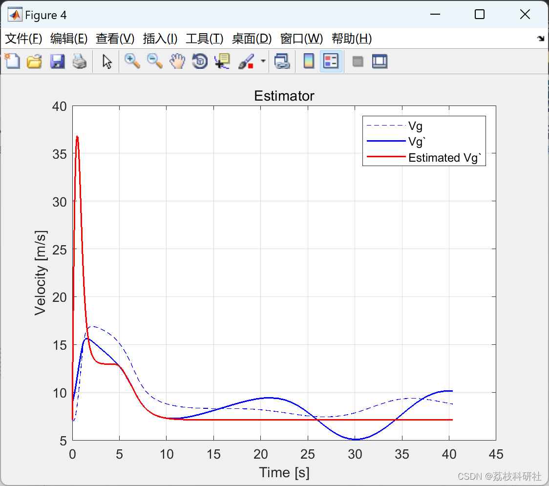
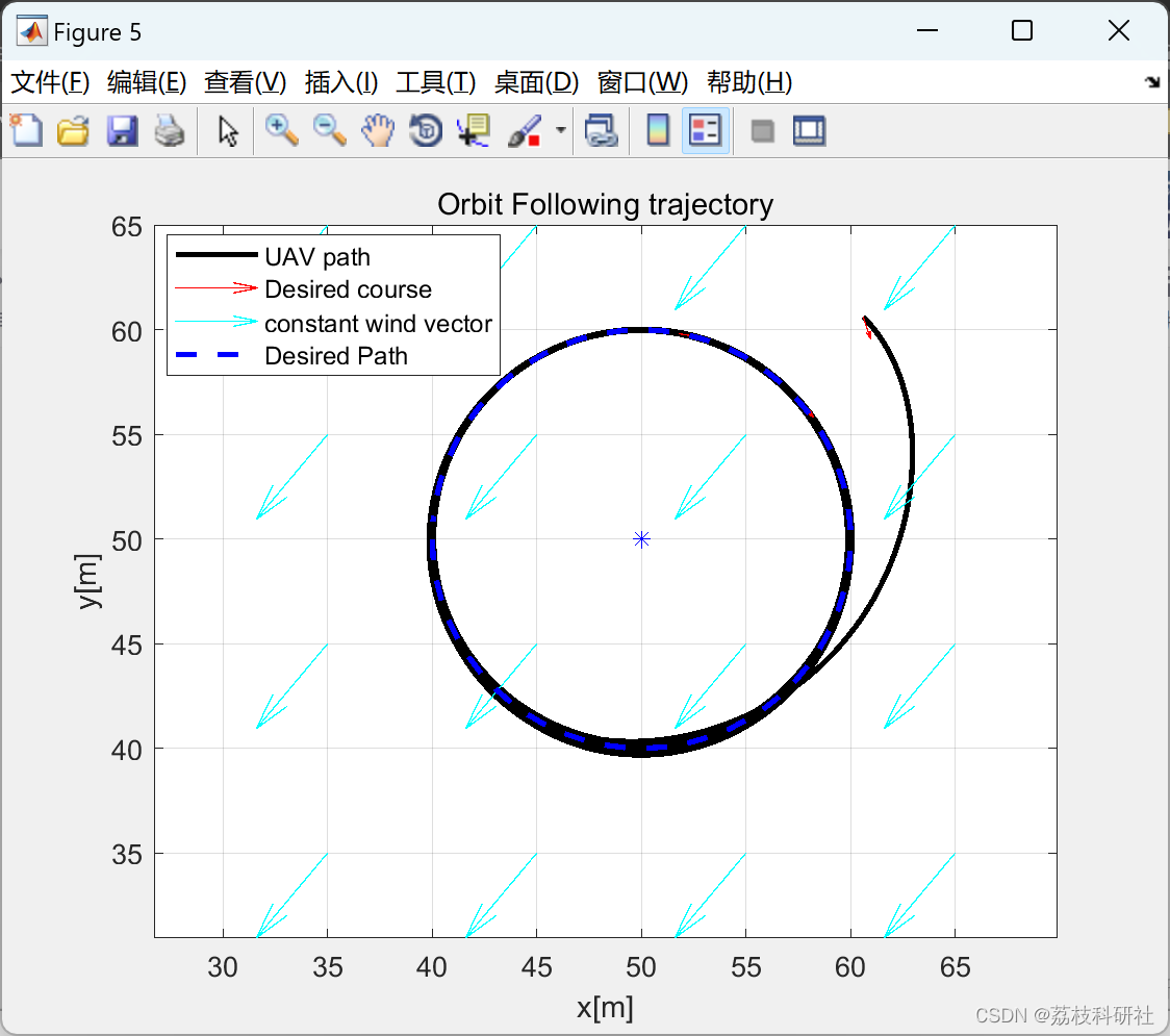
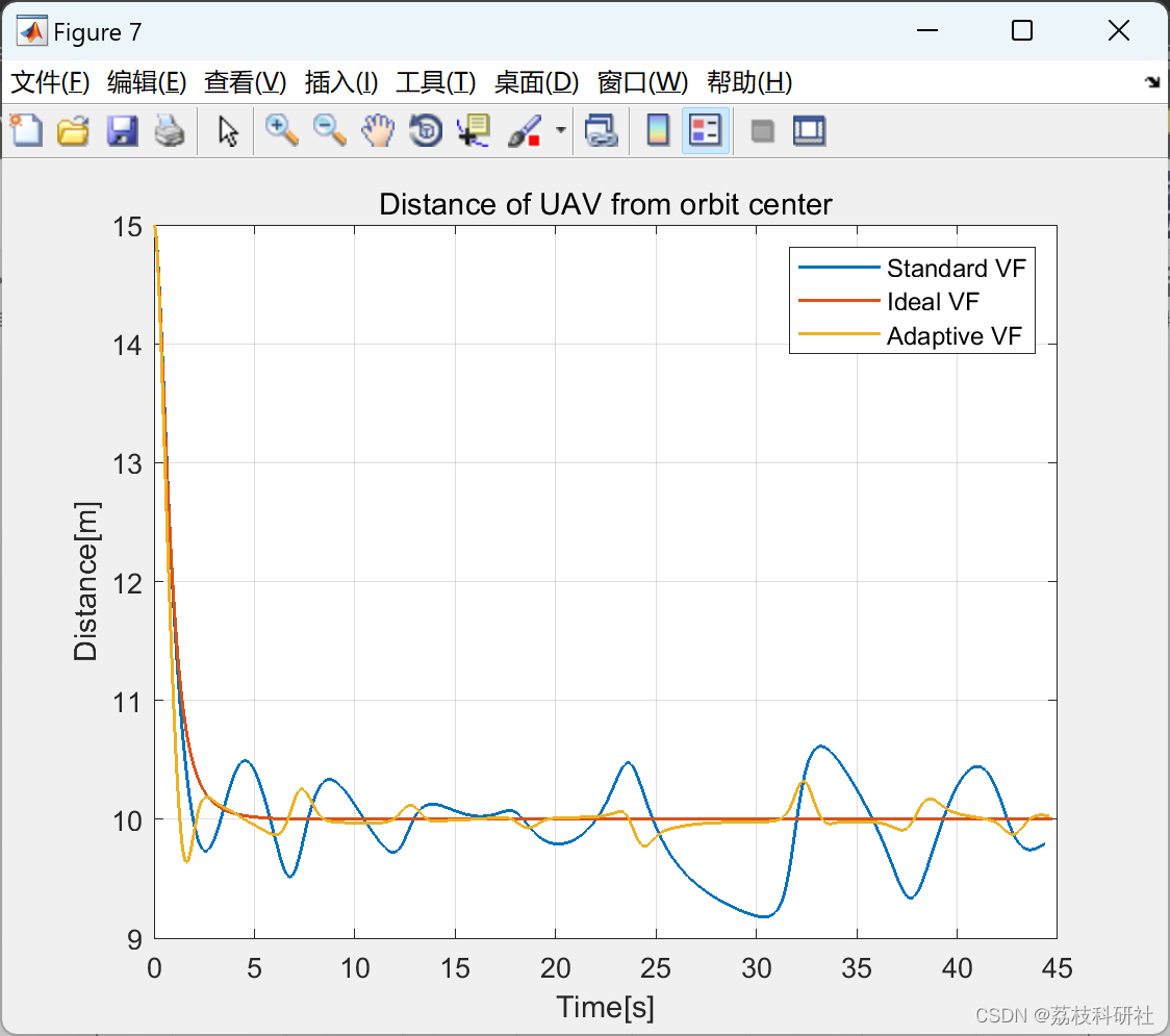
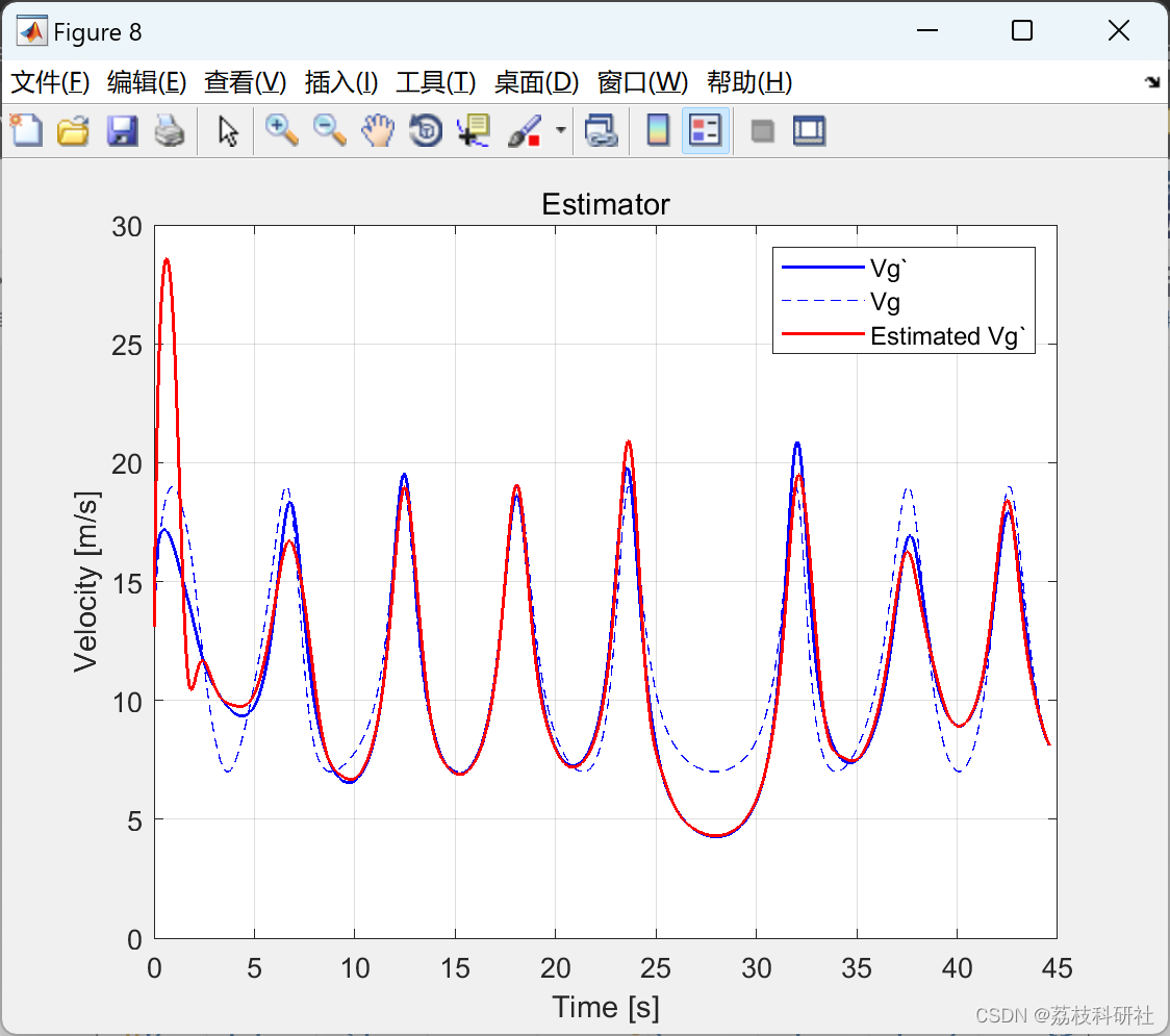
摘要:该文提出一种慢时变风下无人机路径跟随的自适应控制方案。该控制策略将基于矢量场法的路径跟随规律与抵消风未知分量影响的自适应项集成在一起。特别是,结果表明,误差后的路径在缓慢时变的未知风下有界,对于未知恒定风,则收敛为零。数值模拟表明,在风况未知且时变缓慢的环境中,所提方法弥补了对风矢量知识的不足,并且比最先进的矢量场方法获得了更小的误差路径。
原文摘要:
Abstract:
In this paper, an adaptive control scheme for Unmanned Aerial Vehicles (UAVs) path following under slowly time-varying wind is developed. The proposed control strategy integrates the path following law based on the vector field method with an adaptive term counteracting the effect of wind's unknown component. In particular, it is shown that the path following error is bounded under slowly time-varying unknown wind and converges to zero for unknown constant wind. Numerical simulations illustrate that, in environments with unknown and slowly time-varying wind conditions, the proposed method compensates for the lack of knowledge of the wind vector, and attains a smaller path following error than state-of-the-art vector field method.
无人机 (UAV) 在许多应用中用途广泛。应用领域的大多数任务,如对某个目标的军事监视和森林火灾中的救援任务,都依赖于无人机中准确而强大的路径生成器和路径跟踪控制器。路径跟踪控制器设计的挑战源于风干扰、无人机动态特性和传感器质量。本文将风对无人机行为的影响作为路径遵循设计过程中的主要考虑因素。
已经提出几种无人机路径跟踪方法,并在实际无人机平台上进行了测试。在 [1] 中,总结了最先进的 2D 路径跟踪算法,例如胡萝卜追逐算法、非线性制导定律 (NLGL) [2]、基于矢量场 (VF) 的路径跟踪、基于 LQR 的路径跟踪 [3] [4] 和基于视线 (PLOS) 的路径跟踪的纯追踪 [5],并使用两个指标相互比较:总控制工作量和总交叉跟踪误差。
VF路径遵循的基本概念是在所需路径周围构建向量场,以向车辆提供路线命令。通常,路径遵循定律是从李雅普诺夫稳定性分析得出的,该分析保证了全局稳定的收敛到所需路径。这个概念的实现如[6],[7]所示。李雅普诺夫向量场的另一种变体在[8]中提出,称为切向量场引导。
然而,VF方法在完全已知的恒定风扰动的假设下工作。本文的主要贡献是将标准矢量场路径遵循策略[6]扩展到不确定的时变风情景,其中未知和可能的时变风分量可能加起来是一个恒定的风分量。在这项工作中,通过抵消未知风分量影响的估计器来增强路径跟随控制律,从而产生自适应矢量场路径跟随策略。通过Lyapunov方法进行了稳定性分析,结果表明,误差跟随路径在缓慢时变的未知风下有界,对于未知恒风则收敛为零。
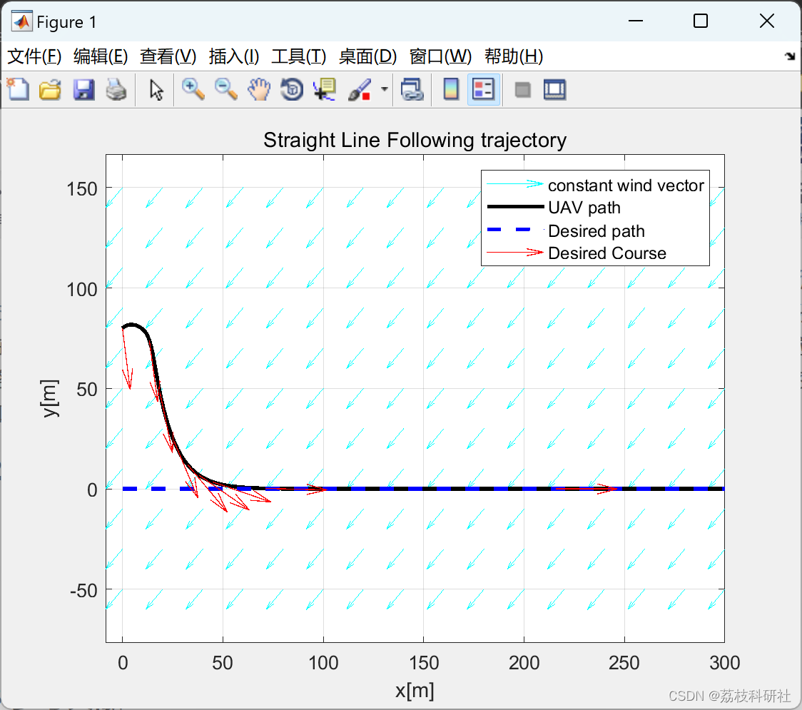
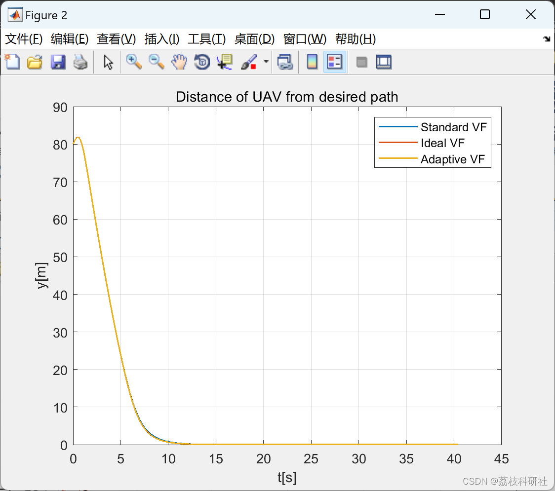
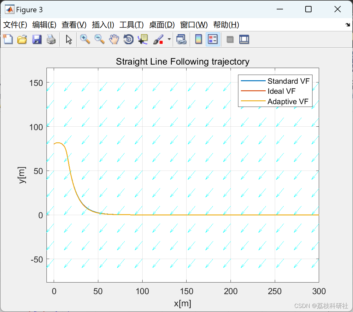
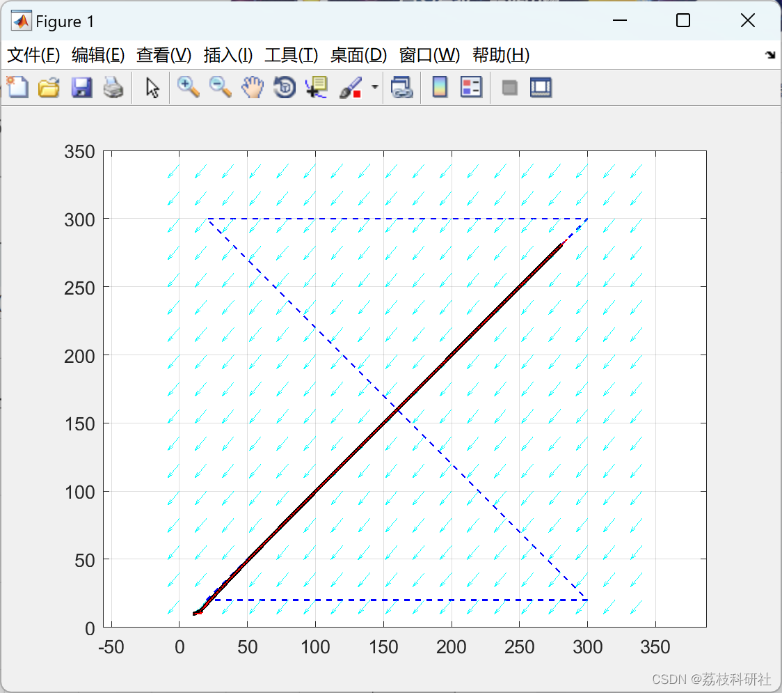
📚2 运行结果

部分代码:
%% Initialization
chi_inf = pi/2; %course angle far away from path (rad)
alpha = 1.65; %positive constant describe the speed of response of course
%hold autopilot loop (rad/s)
k = 0.1; %positive constant influence the rate of the transition from
%x_inf to zero, also control the slope of the
%sliding surface near the origin(m^-1)
kk = pi/2; %gain parameter controls the shape of the trajectories onto
%the sliding surface.(rad^2/s)
epsi = 0.5; %width of the transition region around the sliding surface
%which is used to reduce chattering in the control.(rad)
Gamma = 80; %Estimator gain for straight line
W = 6; %constant wind velocity(m/s)
phiw = 230/180*pi;%constant wind direction(rad)
Va = 13; %Longitudinal velocity(m/s)
A = 3; % Time varying wind's amplitude (variance)
phiA = pi; %Time varying wind's angle (variance)
%% ------------------------------------
% ---------Stright line following------
% -------------------------------------
% Initial conditions
x_int = 0;y_int = 80;course_int = pi/4;%Initial position and posture of UAV
ang = 0; a = 0;b = 0; % Course angle, slop and intercept of desired path
i=-1;% Directon of desired path (i = -1, go right, x increases; i = 1, go left, x decreases)
endx = 300;% stopping condition: the end value of x coordinate
Method =3;% 1: Beard's method, 2: Ideal method, 3: our method
% Initial value of Vg'
Vg0 = InitialVg(A,0,W,phiw,Va,course_int);
% simulation of stright line following
simout=sim('RevisedStraightLine');
% results
figure
[vfx,vfy] = meshgrid(0:20:300,-50:20:150);
wx = W*cos(phiw)*ones(size(vfx));
wy = W*sin(phiw)*ones(size(vfy));
quiver(vfx,vfy,wx,wy,0.5,'c','linewidth',0.5)
hold on
plot(x.data,y.data,'k','linewidth',2)
plot([0 300],[0 0],'--b','linewidth',2)
quiver(x.data(1:50:end),y.data(1:50:end),1*cos(chi_d.data(1:50:end)),1*sin(chi_d.data(1:50:end)),0.4,'r','linewidth',0.5)
🎉3 参考文献
部分理论来源于网络,如有侵权请联系删除。
[1]Bingyu Zhou, H. Satyavada and S. Baldi, "Adaptive path following for Unmanned Aerial Vehicles in time-varying unknown wind environments," 2017 American Control Conference (ACC), Seattle, WA, USA, 2017, pp. 1127-1132, doi: 10.23919/ACC.2017.7963104.


 969
969


 被折叠的 条评论
为什么被折叠?
被折叠的 条评论
为什么被折叠?
 到【灌水乐园】发言


