


机器学习第二十八周周报
摘要
Very Deep Convolutional Networks for Large-Scale Image Recognition,它是由牛津大学计算机视觉组和谷歌一起研究出来的深度卷积神经网络。通常人们所说的VGG是指VGG-16,它由13层卷积层和3层全连接层组成,它有着规律的设计、简洁可堆叠的卷积块,并且在其他数据集上有着很好的表现,因此被人们广泛使用。
Abstract
Very Deep Convolutional Networks for Large-Scale Image Recognition is a deep convolution neural network developed by the computer Vision Group of the University of Oxford and Google. VGG usually refers to VGG-16, which consists of 13 convolution layers and 3 full connection layers. It has regular design, simple and stackable convolution blocks, and has a good performance on other data sets, so it is widely used by people.
一、文献阅读
1.题目
Very Deep Convolutional Networks for Large-Scale Image Recognition
2.Abstract
In this work we investigate the effect of the convolutional network depth on its accuracy in the large-scale image recognition setting. Our main contribution is a thorough evaluation of networks of increasing depth using an architecture with very small (3 × 3) convolution filters, which shows that a significant improvement on the prior-art configurations can be achieved by pushing the depth to 16–19 weight layers. These findings were the basis of our ImageNet Challenge 2014 submission, where our team secured the first and the second places in the localisation and classification tracks respectively. We also show that our representations generalise well to other datasets, where they achieve state-of-the-art results. We have made our two best-performing ConvNet models publicly available to facilitate further research on the use of deep visual representations in computer vision.
在这项工作中,我们研究了卷积网络深度对其在大规模图像识别设置中的准确性的影响。我们的主要贡献是使用一个非常小的(3×3)卷积filter的架构对增加深度的网络进行了彻底的评估,这表明通过将深度提升到16 - 19个weight层,可以显著改善先前的配置。这些发现是我们提交ImageNet挑战赛2014的基础,我们的团队分别获得了本地化和分类的第一名和第二名。我们还展示了我们的成果可以很好地推广到其他数据集,在这些数据集上他们可以得到最优结果。我们已经公开了两个性能最好的卷积神经网络模型,以促进在计算机视觉中使用深度视觉表示的进一步研究。
3.网络结构
(1)结构示意图
VGGNet有以下6种不同的结构,随着层数地增加,结构的深度从左边的A到右边的E逐渐增加(图中为了简洁,没有显示ReLU激活功能)。
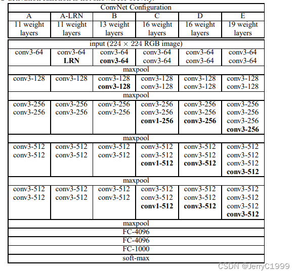
从图中我们可以发现,VGG中卷积层是通过block块相连的,block内部的卷积层结构相同,block之间通过maxpool连接。
图中的conv3-256:卷积层,卷积核尺寸为3,通道数为256。
(2)VGG特点
- VGG-block内的卷积层结构相同,这代表了输入和输出的尺寸相同,并且卷积层可以堆叠复用。
- maxpool层将前一层的卷积层特征缩减一半,使得尺寸缩减规整。
- 深度够深,参数量够大,较深的网络层数使得训练得到的模型分类效果出色,但是较大的参数会对训练和模型保存有更大的资源要求。
- 较小的filter size和kernel size,文献中的kernel size设置为3 * 3。
4.文献解读
(1)Introduction
随着Krizhevsky等人在2012年发表的AlexNet,卷积神经网络在CV领域取得了巨大成功,越来越多的人在其原始架构上进行改进,譬如ILSVRC-2013上效果最好的作品中即选用了较小的感受野尺寸(kernel size较小)和较小的步幅stride;还有2014年的在整个图像上和多尺度下密集训练的网络…而本论文重点讨论了卷积神经网络架构的另一个重要方面:深度。为了使深度更深,作者将架构的其他参数进行了调整,譬如所有卷积层中filter size尺寸都设为很小的3×3,而将卷积层数量加大,使深度更深,事实证明是可行的。
(2)Convnet Configurations
Architecture
在模型训练期间,文献中的预处理是将输入的224 * 224 * 3通道的像素值减去平均RGB值。
图像进入VGG-block块中,fliter size设置为3 * 3,这个尺寸是能捕捉上下左右和中间方位的最小尺寸。
block之间的卷积层stride为1,padding为1,让卷积层层之间尺寸保持一致。
maxpool层stride为2,pool size为2 * 2。
网络中全连接层的配置相同,通过ReLU激活函数进行修正。
VGG的网络结构没有AlexNet中说到的LRN(局部响应正则化),因为作者发现LRN并不能提高性能,反而会带来内存消耗和计算时间地增加。
Configurations
所有的VGG结构都遵从4.2.1里的结构设计,只是其中block内部的卷积层不同。论文中还提到,尽管VGG深度较大,但是相比一些较浅的卷积网络,其参数量并不算很大,因为那些较浅的网络使用filter size很大,以及卷积层的shape较大等。
Discussion
在论文中提到,为什么使用了filter size为3×3叠加卷积层的block,而不是直接用单层的7×7的卷积层?
- 3个卷积层叠加,会有3次relu的非线性校正,比使用1次relu的单层layer更有识别力。
- 降低了参数量,7 * 7 * C * C 比3 * 3 * C * C的参数量大81%。
(3)Classification Framework
参数:batch设为256,动量设为0.9,除最后一层外的全连接层也都使用了丢弃率0.5的dropout,learning rate最初设为0.01,权重衰减系数为5 * 10^(-4)。对于权重层采用了随机初始化,初始化为均值0,方差0.01的正态分布。
论文中提到,为了增加数据集,这里采用了随机水平翻转和随机RGB色差进行数据扩增。对经过重新缩放的图片随机排序并进行随机剪裁得到固定尺寸大小为224 * 224的训练图像。
论文中把S称为training scale,S是经过isotropically-rescaled后的图片的最小边长度。缩放后的图像中只有S>=224的部分才可以被用来做随机剪裁,进行训练。
在论文实现中,采用了两种方式来设定S:
- 固定尺度fix scale:评估了两种scale,S = 256和S = 384。
- 多尺度multi scale:设置了[Smin, Smax]的浮动尺度,范围设为[256, 512]。
(4)Classification Experiments
Single Scale
论文把训练scale和测试的scale分别用S和Q表示;当S为固定值时,令Q = S固定;当S为[Smin,Smax]浮动时,Q固定为 = 0.5[Smin + Smax]。
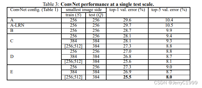
根据上表得到结论:
- 卷积网络总体来说,深度越大,损失越小,效果越好。
- C结果优于B,表明增加非线性relu次数有效。
- D结果优于C,表明了卷积层filter对于捕捉空间特征有帮助。
- E的深度达到19层后,达到了损失的最低点。
- B和同类型filter size为5 * 5的网络进行了对比,发现top-1错误率比B高7%,表明小尺寸filter效果更好。
- 在训练中,采用浮动尺度效果更好,因为这有助于学习分类目标在不同尺寸下的特征。
Multi Scale
当训练时的S固定时,Q取{S - 32, S, S+32}中的每个值,进行测试过后取平均结果。 当S为[Smin,Smax]浮动时,Q取{Smin, 0.5(Smin+Smax), Smax},测试后取平均。
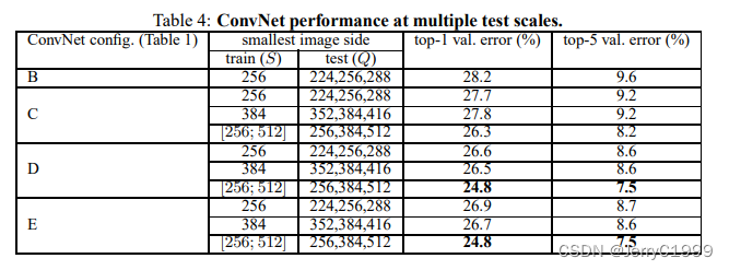
根据上表得到结论:
- 模型深度越深,效果越好。
- 同样的深度下,浮动scale效果优于固定scale。
(5)Conclusion
作者总结:我们评估了非常深的卷积网络(多达19权重层)的大规模图像分类。 研究表明,表征深度有利于分类的准确性,并且可以通过使用传统的 ConvNet 架构在 ImageNet 挑战数据集上的最先进的性能。
二、深度学习
1.CNN卷积神经网络的5个层级结构
输入层
模型需要输入进行预处理操作,常见的输入层中预处理方式有:去均值、归一化、PCA/SVD降维等。
卷积层
卷积层的作用:
- 提取图像的特征,并且卷积核的权重是可以学习的,由此在高层神经网络中,卷积操作能够突破传统滤波器的限制,根据目标函数提取出想要的特征。
- 局部感知,参数共享,大大降低了网络参数,保证了网络的稀疏性,防止过拟合。
激活层
激活层实际上就是对卷积层的输出结果做一次非线性映射,优点是进行特征提取时,为了使数据量小,操作方便,就可以舍弃掉一些没有关联的数据。
池化层
池化层的作用:
池化层可以对提取到的特征信息进行降维,一方面使特征图变小,简化网络计算复杂度并在一定程度上避免过拟合的出现;另一方面进行特征压缩,提取主要特征。
全连接层
全连接层是对特征图进行维度上的改变,以此得到每个类别对应的概率。
在全连接层之前,如果神经元数目过大,学习能力强,有可能出现过拟合。因此,可以引入dropout操作,来随机删除神经网络中的部分神经元,正则化等以此解决问题。
2.CNN手写数字识别
定义训练的设备
import time

import numpy as np
import torch
from torch import nn
from PIL import Image
import matplotlib.pyplot as plt
import os
import torch.nn.functional as F

from torch.utils.data import DataLoader
from torch.utils.tensorboard import SummaryWriter
from torchvision import datasets, transforms, utils

device = torch.device("cuda" if torch.cuda.is_available() else "cpu")
print(device)
准备MNIST数据集
transform = transforms.Compose([transforms.ToTensor(),
                                transforms.Normalize(mean=[0.5], std=[0.5])])

train_data = datasets.MNIST(root="../data", train=True, transform=transform, download=True)

test_data = datasets.MNIST(root="../data", train=False, transform=transform, download=True)
利用 DataLoader 来加载MNIST数据集
train_dataloader = DataLoader(train_data, batch_size=32, shuffle=True, pin_memory=True)
test_dataloader = DataLoader(test_data, batch_size=32, shuffle=True)
创建CNN网络模型
class CNN(nn.Module):
    def __init__(self):
        super(CNN, self).__init__()
        self.conv1 = nn.Conv2d(1, 6, 5)
        self.conv2 = nn.Conv2d(6, 16, 5)
        self.fc1 = nn.Linear(16 * 4 * 4, 120)
        self.fc2 = nn.Linear(120, 84)
        self.fc3 = nn.Linear(84, 10)

    def forward(self, x):

        x = F.relu(self.conv1(x))
        x = F.max_pool2d(x, 2, 2)
        x = F.relu(self.conv2(x))
        x = F.max_pool2d(x, 2, 2)
        x = x.view(x.shape[0], -1)
        x = F.relu(self.fc1(x))
        x = F.relu(self.fc2(x))
        x = self.fc3(x)
        return F.log_softmax(x, dim=1)


net = CNN()
net = net.to(device)
定义损失函数和优化器
loss_fn = nn.CrossEntropyLoss()
loss_fn = loss_fn.to(device)

learning_rate = 1e-2
optimizer = torch.optim.SGD(net.parameters(), lr=learning_rate, momentum=0.5)
设置训练网络的一些参数:记录训练的次数、记录测试的次数和训练的轮数。
添加tensorboard,对训练和测试的loss可视化,以及测试准确率可视化。
total_train_step = 0
total_test_step = 0
epoch = 10

writer = SummaryWriter("../logs_train")
start_time = time.time()
模型的训练和测试
for i in range(epoch):
    print("--------第 {} 轮训练开始--------".format(i + 1))

    # 训练步骤开始
    net.train()
    for data in train_dataloader:
        imgs, targets = data
        imgs = imgs.to(device)
        targets = targets.to(device)
        ouputs = net(imgs)
        loss = loss_fn(ouputs, targets)

        # 优化器优化模型
        optimizer.zero_grad()
        loss.backward()
        optimizer.step()

        total_train_step = total_train_step + 1
        if total_train_step % 100 == 0:
            end_time = time.time()
            print(end_time - start_time)
            print("训练次数:{},Loss:{}".format(total_train_step, loss.item()))
            writer.add_scalar("train_loss", loss.item(), total_train_step)

    # 测试步骤开始
    net.eval()
    total_test_loss = 0
    total_accuracy = 0
    with torch.no_grad():
        for data in test_dataloader:
            imgs, targets = data
            imgs = imgs.to(device)
            targets = targets.to(device)
            ouputs = net(imgs)

            loss = loss_fn(ouputs, targets)
            total_test_loss = total_test_loss + loss
            accuracy = (ouputs.argmax(1) == targets).sum()
            total_accuracy = total_accuracy + accuracy

        print("整体测试集上的Loss:{}".format(total_test_loss))
        print("整体测试集上的正确率:{}".format(total_accuracy / test_data_size))
        writer.add_scalar("test_loss", total_test_loss, total_test_step)
        writer.add_scalar("test_accuracy", total_accuracy / test_data_size, total_test_step)
        total_test_step = total_test_step + 1

        torch.save(net, "net_{}.pth".format(i))
        print("模型已保存")

writer.close()
对模型进行验证,测试模型的正确率。
import torch
from torchvision import datasets, transforms, utils
from PIL import Image
from torch import nn
import torch.nn.functional as F

image_path = "../imgs/three.jpg"
image = Image.open(image_path)
if image.mode != 'L':
    image = image.convert('L')
print(image)

transform = transforms.Compose([transforms.ToTensor(),
                                transforms.Normalize(mean=[0.5], std=[0.5]),
                                transforms.Resize((28, 28))])

image = transform(image)
print(image.shape)


class CNN(nn.Module):
    def __init__(self):
        super(CNN, self).__init__()
        self.conv1 = nn.Conv2d(1, 6, 5)
        self.conv2 = nn.Conv2d(6, 16, 5)
        self.fc1 = nn.Linear(16 * 4 * 4, 120)
        self.fc2 = nn.Linear(120, 84)
        self.fc3 = nn.Linear(84, 10)

    def forward(self, x):
        x = F.relu(self.conv1(x))
        x = F.max_pool2d(x, 2, 2)
        x = F.relu(self.conv2(x))
        x = F.max_pool2d(x, 2, 2)
        x = x.view(x.shape[0], -1)
        x = F.relu(self.fc1(x))
        x = F.relu(self.fc2(x))
        x = self.fc3(x)
        return F.log_softmax(x, dim=1)


model = torch.load("net_0.pth", map_location=torch.device('cpu'))
print(model)

image = torch.reshape(image, (1, 1, 28, 28))
model.eval()
with torch.no_grad():
    output = model(image)
print(output)
print(output.argmax(1))
通过数据集和输出结果比对,验证成功。
<PIL.Image.Image image mode=L size=499x500 at 0x185642FAA30>
torch.Size([1, 28, 28])
CNN(
  (conv1): Conv2d(1, 6, kernel_size=(5, 5), stride=(1, 1))
  (conv2): Conv2d(6, 16, kernel_size=(5, 5), stride=(1, 1))
  (fc1): Linear(in_features=256, out_features=120, bias=True)
  (fc2): Linear(in_features=120, out_features=84, bias=True)
  (fc3): Linear(in_features=84, out_features=10, bias=True)
)
tensor([[ -6.2694, -11.1973,  -4.3984,  -0.4182,  -7.2111,  -3.6906, -10.5494,
          -3.5908,  -5.5567,  -1.3079]])
tensor([3])
MNIST数据集,从二维数组生成一张图片。
img, label = train_data[0]
img = img.numpy().transpose(1, 2, 0)
std = [0.5]
mean = [0.5]
img = img * std + mean
plt.imshow(img)
plt.show()
三、总结
VGGNet通过在传统卷积神经网络模型上进行拓展,除了较为复杂的模型结构设计以外,发现深度对于提高模型准确率非常重要。VGG深度更深,参数量更大,效果和可移植性更好,模型设计简洁且规律,固而被广泛使用。下周会继续阅读CNN相关文献,提升自己对CNN的深入理解。


 1282
1282


 被折叠的 条评论
为什么被折叠?
被折叠的 条评论
为什么被折叠?
 到【灌水乐园】发言


