


regularization_linear_regression.py
import numpy as np
import matplotlib.pyplot as plt


class RegularizationLinearRegression:
    """
    线性回归 + 正则化,梯度下降法 + 闭式解求解模型系数
    1、数据的预处理:是否训练偏置项fit_intercept(默认True),是否标准化normalized(默认True)
    2、模型的训练:fit(self, x_train, y_train):闭式解form,梯度下降法:grad
    3、模型的预测,predict(self, x_test)
    4、均方误差,判决系数
    5、模型预测可视化
    """

    def __init__(self, solver="grad", fit_intercept=True, normalize=True, alpha=0.05,
                 max_epochs=300, batch_size=20, l1_ratio=None, l2_ratio=None, en_rou=None):
        """
        :param solver: 求解方法:form是闭式解,grad是梯度
        :param fit_intercept: 是否训练偏置项
        :param normalize: 是否标准化
        :param alpha: 学习率
        :param max_epochs: 最大迭代次数
        :param batch_size: 批量大小,若为1,则为随机梯度,若为训练集样本量,则为批量梯度,否则为小批量梯度
        :param l1_ratio: LASSO回归惩罚项系数
        :param l2_ratio: 岭回归惩罚项系数
        :param en_rou: 弹性网络权衡L1和L2的系数
        """
        self.solver = solver  # 求解方法
        self.fit_intercept = fit_intercept  # 线性模型的常数项。也即偏置bias,模型中的theta0
        self.normalize = normalize  # 是否标准化数据
        self.alpha = alpha  # 学习率
        if l1_ratio:
            if l1_ratio < 0:
                raise ValueError("惩罚项系数不能为负数")
        self.l1_ratio = l1_ratio  # LASSO回归惩罚项系数
        if l2_ratio:
            if l2_ratio < 0:
                raise ValueError("惩罚项系数不能为负数")
        self.l2_ratio = l2_ratio  # 岭回归惩罚项系数
        if en_rou:
            if en_rou > 1 or en_rou < 0:
                raise ValueError("弹性网络权衡系数范围在[0, 1]")
        self.en_rou = en_rou  # 弹性网络权衡L1和L2的系数
        self.max_epochs = max_epochs
        self.batch_size = batch_size
        self.theta = None  # 训练权重系数
        if normalize:
            self.feature_mean, self.feature_std = None, None  # 特征的均值,标准方差
        self.mse = np.infty  # 训练样本的均方误差
        self.r2, self.r2_adj = 0.0, 0.0  # 判定系数和修正判定系数
        self.n_samples, self.n_features = 0, 0  # 样本量和特征数
        self.train_loss, self.test_loss = [], []  # 存储训练过程中的训练损失和测试损失

    def init_params(self, n_features):
        """
        初始化参数
        如果训练偏置项,也包含了bias的初始化
        :return:
        """
        self.theta = np.random.randn(n_features, 1) * 0.1

    def fit(self, x_train, y_train, x_test=None, y_test=None):
        """
        样本的预处理,模型系数的求解,闭式解公式 + 梯度方法
        :param x_train: 训练样本集 m*k
        :param y_train: 训练目标集 m*1
        :param x_test: 测试样本集 n*k
        :param y_test: 测试目标集 n*1
        :return:
        """
        if self.normalize:
            self.feature_mean = np.mean(x_train, axis=0)  # 样本均值
            self.feature_std = np.std(x_train, axis=0) + 1e-8  # 样本方差
            x_train = (x_train - self.feature_mean) / self.feature_std  # 标准化
            if x_test is not None:
                x_test = (x_test - self.feature_mean) / self.feature_std  # 标准化
        if self.fit_intercept:
            x_train = np.c_[x_train, np.ones_like(y_train)]  # 添加一列1,即偏置项样本
            if x_test is not None and y_test is not None:
                x_test = np.c_[x_test, np.ones_like(y_test)]  # 添加一列1,即偏置项样本
        self.init_params(x_train.shape[1])  # 初始化参数
        # 训练模型
        if self.solver == "grad":
            self._fit_gradient_desc(x_train, y_train, x_test, y_test)  # 梯度下降法训练模型
        elif self.solver == "form":
            self._fit_closed_form_solution(x_train, y_train)
        else:
            raise ValueError("仅限于闭式解form或梯度下降算法grad")

    def _fit_closed_form_solution(self, x_train, y_train):
        """
        线性回归的闭式解,单独函数,以便后期扩充维护
        :param x_train: 训练样本集
        :param y_train: 训练目标集
        :return:
        """
        # pinv伪逆,即(A^T * A)^(-1) * A^T
        if self.l2_ratio is None:
            self.theta = np.linalg.pinv(x_train).dot(y_train)  # 非正则化
            # xtx = np.dot(x_train.T, x_train) + 0.01 * np.eye(x_train.shape[1])  # 按公式书写
            # self.theta = np.dot(np.linalg.inv(xtx), x_train.T).dot(y_train)
        elif self.l2_ratio:
            self.theta = np.linalg.inv(x_train.T.dot(x_train) + self.l2_ratio *
                                       np.eye(x_train.shape[1])).dot(x_train.T).dot(y_train)
        else:
            pass

    def _fit_gradient_desc(self, x_train, y_train, x_test=None, y_test=None):
        """
        三种梯度下降求解 + 正则化:
        (1)如果batch_size为1,则为随机梯度下降法
        (2)如果batch_size为样本量,则为批量梯度下降法
        (3)如果batch_size小于样本量,则为小批量梯度下降法
        :return:
        """
        train_sample = np.c_[x_train, y_train]  # 组合训练集和目标集,以便随机打乱样本
        # np.c_水平方向连接数组,np.r_竖直方向连接数组
        # 按batch_size更新theta,三种梯度下降法取决于batch_size的大小
        best_theta, best_mse = None, np.infty  # 最佳训练权重与验证均方误差
        for i in range(self.max_epochs):
            self.alpha *= 0.95
            np.random.shuffle(train_sample)  # 打乱样本顺序,模拟随机化
            batch_nums = train_sample.shape[0] // self.batch_size  # 批次
            for idx in range(batch_nums):
                # 取小批量样本,可以是随机梯度(1),批量梯度(n)或者是小批量梯度(<n)
                batch_xy = train_sample[self.batch_size * idx: self.batch_size * (idx + 1)]
                # 分取训练样本和目标样本,并保持维度
                batch_x, batch_y = batch_xy[:, :-1], batch_xy[:, -1:]
                # 计算权重更新增量,包含偏置项
                delta = batch_x.T.dot(batch_x.dot(self.theta) - batch_y) / self.batch_size
                # 计算并添加正则化部分,不包含偏置项
                dw_reg = np.zeros(shape=(x_train.shape[1] - 1, 1))
                if self.l1_ratio and self.l2_ratio is None:
                    # LASSO回归,L1正则化
                    dw_reg = self.l1_ratio * np.sign(self.theta[:-1]) / self.batch_size
                if self.l2_ratio and self.l1_ratio is None:
                    dw_reg = 2 * self.l2_ratio * self.theta[:-1] / self.batch_size
                if self.en_rou and self.l1_ratio and self.l2_ratio:
                    dw_reg = self.l1_ratio * self.en_rou * np.sign(self.theta[:-1]) / self.batch_size
                    dw_reg += 2 * self.l2_ratio * (1 - self.en_rou) * self.theta[:-1] / self.batch_size
                delta[:-1] += dw_reg  # 添加了正则化
                self.theta = self.theta - self.alpha * delta
            train_mse = ((x_train.dot(self.theta) - y_train.reshape(-1, 1)) ** 2).mean()
            self.train_loss.append(train_mse)
            if x_test is not None and y_test is not None:
                test_mse = ((x_test.dot(self.theta) - y_test.reshape(-1, 1)) ** 2).mean()
                self.test_loss.append(test_mse)

    def get_params(self):
        """
        返回线性模型训练的系数
        :return:
        """
        if self.fit_intercept:  # 存在偏置项
            weight, bias = self.theta[:-1], self.theta[-1]
        else:
            weight, bias = self.theta, np.array([0])
        if self.normalize:  # 标准化后的系数
            weight = weight / self.feature_std.reshape(-1, 1)  # 还原模型系数
            bias = bias - weight.T.dot(self.feature_mean)
        return weight.reshape(-1), bias

    def predict(self, x_test):
        """
        测试数据预测
        :param x_test: 待预测样本集,不包括偏置项
        :return:
        """
        try:
            self.n_samples, self.n_features = x_test.shape[0], x_test.shape[1]
        except IndexError:
            self.n_samples, self.n_features = x_test.shape[0], 1  # 测试样本数和特征数
        if self.normalize:
            x_test = (x_test - self.feature_mean) / self.feature_std  # 测试数据标准化
        if self.fit_intercept:
            # 存在偏置项,加一列1
            x_test = np.c_[x_test, np.ones(shape=x_test.shape[0])]
        y_pred = x_test.dot(self.theta).reshape(-1, 1)
        return y_pred

    def cal_mse_r2(self, y_test, y_pred):
        """
        计算均方误差,计算拟合优度的判定系数R方和修正判定系数
        :param y_pred: 模型预测目标真值
        :param y_test: 测试目标真值
        :return:
        """
        self.mse = ((y_test.reshape(-1, 1) - y_pred.reshape(-1, 1)) ** 2).mean()  # 均方误差
        # 计算测试样本的判定系数和修正判定系数
        self.r2 = 1 - ((y_test.reshape(-1, 1) - y_pred.reshape(-1, 1)) ** 2).sum() / \
                  ((y_test.reshape(-1, 1) - y_test.mean()) ** 2).sum()
        self.r2_adj = 1 - (1 - self.r2) * (self.n_samples - 1) / \
                      (self.n_samples - self.n_features - 1)
        return self.mse, self.r2, self.r2_adj

    def plt_predict(self, y_test, y_pred, is_show=True, is_sort=True):
        """
        绘制预测值与真实值对比图
        :return:
        """
        if self.mse is np.infty:
            self.cal_mse_r2(y_pred, y_test)
        if is_show:
            plt.figure(figsize=(8, 6))
        if is_sort:
            idx = np.argsort(y_test)  # 升序排列,获得排序后的索引
            plt.plot(y_test[idx], "k--", lw=1.5, label="Test True Val")
            plt.plot(y_pred[idx], "r:", lw=1.8, label="Predictive Val")
        else:
            plt.plot(y_test, "ko-", lw=1.5, label="Test True Val")
            plt.plot(y_pred, "r*-", lw=1.8, label="Predictive Val")
        plt.xlabel("Test sample observation serial number", fontdict={"fontsize": 12})
        plt.ylabel("Predicted sample value", fontdict={"fontsize": 12})
        plt.title("The predictive values of test samples \n MSE = %.5e, R2 = %.5f, R2_adj = %.5f"
                  % (self.mse, self.r2, self.r2_adj), fontdict={"fontsize": 14})
        plt.legend(frameon=False)
        plt.grid(ls=":")
        if is_show:
            plt.show()

    def plt_loss_curve(self, is_show=True):
        """
        可视化均方损失下降曲线
        :param is_show: 是否可视化
        :return:
        """
        if is_show:
            plt.figure(figsize=(8, 6))
        plt.plot(self.train_loss, "k-", lw=1, label="Train Loss")
        if self.test_loss:
            plt.plot(self.test_loss, "r--", lw=1.2, label="Test Loss")
        plt.xlabel("Epochs", fontdict={"fontsize": 12})
        plt.ylabel("Loss values", fontdict={"fontsize": 12})
        plt.title("Gradient Descent Method and Test Loss MSE = %.5f"
                  % (self.test_loss[-1]), fontdict={"fontsize": 14})
        plt.legend(frameon=False)
        plt.grid(ls=":")
        # plt.axis([0, 300, 20, 30])
        if is_show:
            plt.show()
test_reg_linear_regression.py
import matplotlib.pyplot as plt
import numpy as np
from polynomial_feature import PolynomialFeatureData
from regularization_linear_regression import RegularizationLinearRegression
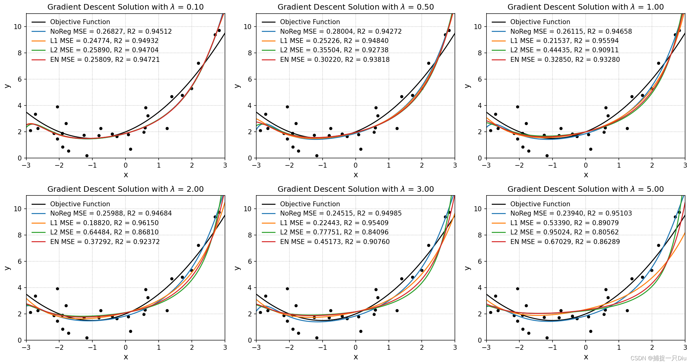
def objective_fun(x):
"""
目标函数
:param x:
:return:
"""
return 0.5 * x ** 2 + x + 2
np.random.seed(42)
n = 30 # 采样数据的样本量
raw_x = np.sort(6 * np.random.rand(n, 1) - 3, axis=0) # [-3, 3]区间,排序,二维数组n * 1
raw_y = objective_fun(raw_x) + np.random.randn(n, 1) # 二维数组
feature_obj = PolynomialFeatureData(raw_x, degree=13, with_bias=False)
X_train = feature_obj.fit_transform() # 特征数据的构造
X_test_raw = np.linspace(-3, 3, 150) # 测试数据
feature_obj = PolynomialFeatureData(X_test_raw, degree=13, with_bias=False)
X_test = feature_obj.fit_transform() # 特征数据的构造
y_test = objective_fun(X_test_raw) # 测试样本的真值
reg_ratio = [0.1, 0.5, 1, 2, 3, 5] # 正则化系数
alpha, batch_size, max_epochs = 0.1, 10, 300
plt.figure(figsize=(15, 8))
for i, ratio in enumerate(reg_ratio):
plt.subplot(231 + i)
# 不采用正则化
reg_lr = RegularizationLinearRegression(solver="grad", alpha=alpha, batch_size=batch_size,
max_epochs=max_epochs)
reg_lr.fit(X_train, raw_y)
print("NoReg, ratio = 0.00", reg_lr.get_params())
print("=" * 70)
y_test_pred = reg_lr.predict(X_test) # 测试样本预测
mse, r2, _ = reg_lr.cal_mse_r2(y_test, y_test_pred)
plt.scatter(raw_x, raw_y, s=15, c="k")
plt.plot(X_test_raw, y_test, "k-", lw=1.5, label="Objective Function")
plt.plot(X_test_raw, y_test_pred, lw=1.5, label="NoReg MSE = %.5f, R2 = %.5f" % (mse, r2))
# LASSO回归
# LASSO: Least absolute shrinkage and selection operator 最小绝对收缩与选择算子
lasso_lr = RegularizationLinearRegression(solver="grad", alpha=alpha, batch_size=batch_size,
max_epochs=max_epochs, l1_ratio=ratio)
lasso_lr.fit(X_train, raw_y)
print("L1, ratio = %.2f" % ratio, lasso_lr.get_params())
print("=" * 70)
y_test_pred = lasso_lr.predict(X_test) # 测试样本预测
mse, r2, _ = lasso_lr.cal_mse_r2(y_test, y_test_pred)
plt.plot(X_test_raw, y_test_pred, lw=1.5, label="L1 MSE = %.5f, R2 = %.5f" % (mse, r2))
# 岭回归
ridge_lr = RegularizationLinearRegression(solver="grad", alpha=alpha, batch_size=batch_size,
max_epochs=max_epochs, l2_ratio=ratio)
ridge_lr.fit(X_train, raw_y)
print("L2, ratio = %.2f" % ratio, ridge_lr.get_params())
print("=" * 70)
y_test_pred = ridge_lr.predict(X_test) # 测试样本预测
mse, r2, _ = ridge_lr.cal_mse_r2(y_test, y_test_pred)
plt.plot(X_test_raw, y_test_pred, lw=1.5, label="L2 MSE = %.5f, R2 = %.5f" % (mse, r2))
# 弹性网络回归
elastic_net_lr = RegularizationLinearRegression(solver="grad", alpha=alpha, batch_size=batch_size,
max_epochs=max_epochs, l2_ratio=ratio, l1_ratio=ratio, en_rou=0.5)
elastic_net_lr.fit(X_train, raw_y)
print("EN, ratio = %.2f" % ratio, elastic_net_lr.get_params())
print("=" * 70)
y_test_pred = elastic_net_lr.predict(X_test) # 测试样本预测
mse, r2, _ = elastic_net_lr.cal_mse_r2(y_test, y_test_pred)
plt.plot(X_test_raw, y_test_pred, lw=1.5, label="EN MSE = %.5f, R2 = %.5f" % (mse, r2))
plt.axis([-3, 3, 0, 11])
plt.xlabel("x", fontdict={"fontsize": 12})
plt.ylabel("y", fontdict={"fontsize": 12})
plt.legend(frameon=False)
plt.grid(ls=":")
#plt.title("Closed Form Solution with $\lambda$ = %.2f" % ratio)
plt.title("Gradient Descent Solution with $\lambda$ = %.2f" % ratio)
plt.tight_layout()
plt.show()

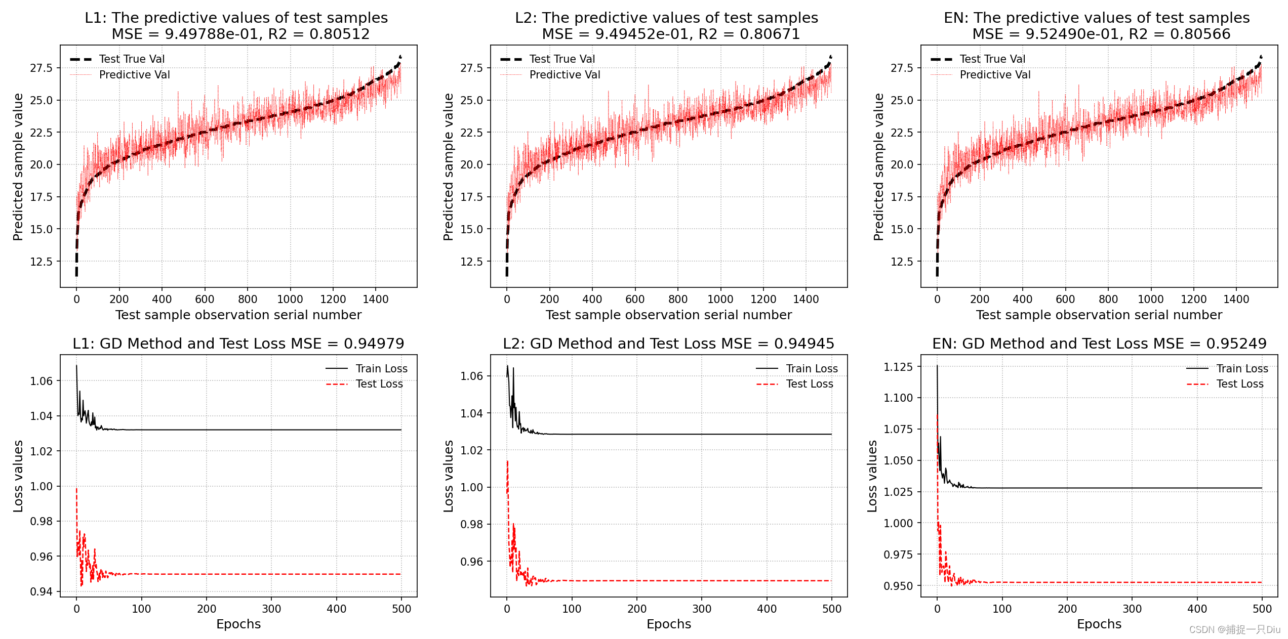
案例测试
http://archive.ics.uci.edu/ml/datasets/Bias+correction+of+numerical+prediction+model+temperature+forecast
import matplotlib.pyplot as plt
import numpy as np
import pandas as pd
from regularization_linear_regression import RegularizationLinearRegression
from sklearn.model_selection import train_test_split


data = pd.read_csv("bias+correction+of+numerical+prediction+model+temperature+forecast/Bias_correction_ucl.csv").dropna()
X, y = np.asarray(data.iloc[:, 2:-2]), np.asarray(data.iloc[:, -1])
feature_names = data.columns[2:-2]

X_train, X_test, y_train, y_test = train_test_split(X, y, test_size=0.2, random_state=22)
alpha, batch_size, max_epochs, ratio = 0.2, 100, 500, 0.5

plt.figure(figsize=(15, 8))

noreg_lr = RegularizationLinearRegression(alpha=alpha, batch_size=batch_size, max_epochs=max_epochs)
noreg_lr.fit(X_train, y_train)
theta = noreg_lr.get_params()
print("无正则化,模型系数如下")
for i, w in enumerate(theta[0][:-1]):
    print(feature_names[i], ":", w)
print("theta0:", theta[1][0])
print("=" * 50)

lasso_lr = RegularizationLinearRegression(alpha=alpha, batch_size=batch_size, max_epochs=max_epochs, l1_ratio=1)
lasso_lr.fit(X_train, y_train, X_test, y_test)
theta = lasso_lr.get_params()
print("LASSO正则化,模型系数如下")
for i, w in enumerate(theta[0][:-1]):
    print(feature_names[i], ":", w)
print("theta0:", theta[1][0])
print("=" * 50)
plt.subplot(231)
y_test_pred = lasso_lr.predict(X_test)  # 测试样本预测
lasso_lr.plt_predict(y_test, y_test_pred, lab="L1", is_sort=True, is_show=False)
plt.subplot(234)
lasso_lr.plt_loss_curve(lab="L1", is_show=False)


ridge_lr = RegularizationLinearRegression(alpha=alpha, batch_size=batch_size, max_epochs=max_epochs, l1_ratio=ratio)
ridge_lr.fit(X_train, y_train, X_test, y_test)
theta = ridge_lr.get_params()
print("岭回归正则化,模型系数如下")
for i, w in enumerate(theta[0][:-1]):
    print(feature_names[i], ":", w)
print("theta0:", theta[1][0])
print("=" * 50)
plt.subplot(232)
y_test_pred = ridge_lr.predict(X_test)  # 测试样本预测
ridge_lr.plt_predict(y_test, y_test_pred, lab="L2", is_sort=True, is_show=False)
plt.subplot(235)
ridge_lr.plt_loss_curve(lab="L2", is_show=False)


en_lr = RegularizationLinearRegression(alpha=alpha, batch_size=batch_size, max_epochs=max_epochs,
                                       l1_ratio=ratio, l2_ratio=ratio, en_rou=0.3)
en_lr.fit(X_train, y_train, X_test, y_test)
theta = en_lr.get_params()
print("弹性网络正则化,模型系数如下")
for i, w in enumerate(theta[0][:-1]):
    print(feature_names[i], ":", w)
print("theta0:", theta[1][0])
print("=" * 50)
plt.subplot(233)
y_test_pred = en_lr.predict(X_test)  # 测试样本预测
en_lr.plt_predict(y_test, y_test_pred, lab="EN", is_sort=True, is_show=False)
plt.subplot(236)
en_lr.plt_loss_curve(lab="EN", is_show=False)

plt.tight_layout()
plt.show()


 2078
2078


 被折叠的 条评论
为什么被折叠?
被折叠的 条评论
为什么被折叠?
 到【灌水乐园】发言


