NeRF PyTorch 源码解读

对 NeRF PyTorch 的源码进行解读，代码链接： https://github.com/yenchenlin/nerf-pytorch。NeRF 的整体流程如下：

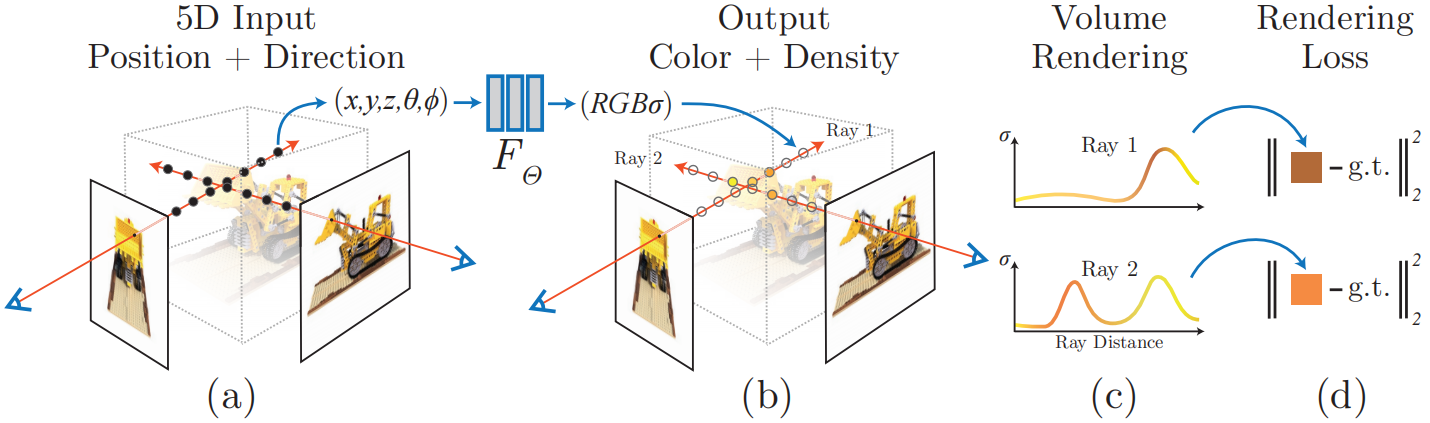
图片来源于文献： NeRF: Representing Scenes as Neural Radiance Fields for View Synthesis

一、数据集加载

以 load_llff_data 为例，对代码中的数据集加载流程进行分析。

1. LLFF 数据集

LLFF数据集的官方链接：https://github.com/Fyusion/LLFF。关于 LLFF 中 poses_bounds.npy 的介绍如下：

总结一下上面的描述：

• poses_bounds.npy 包括 $N\times 17$ 的 NumPy 数组，每行有 17 个元素，其中前 12 个表示相机坐标系到世界坐标系的旋转矩阵和平移向量，第 13 到 第 15 个元素表示图像的宽和高以及相机的焦距，最后两位数值表示近平面和远平面；
• LLFF 的坐标系是 DRB，即 $X$ 轴向下、$Y$ 轴向右、$Z$ 轴向后，这与 COLMAP 坐标系和 NeRF 坐标系不一致；
• 在 LLFF 中，默认图像平面的原点位于像素平面的中心处，并且 $f=f_x=f_y$。

2. _load_data 函数

poses_arr = np.load(os.path.join(basedir, 'poses_bounds.npy'))
# 例: pose[:, :, 0] = [R, T, img_info], R 为 3x3 的旋转矩阵, T 为 3x1 的平移向量，img_info 为 3x1 的向量 (H, W, f)^T
poses = poses_arr[:, :-2].reshape([-1, 3, 5]).transpose([1, 2, 0])  # (N, 15) -> (N, 3, 5) -> (3, 5, N)
bds = poses_arr[:, -2:].transpose([1, 0])  # (N, 2) -> (2, N)，bds 存储着近平面和远平面的数值

poses_bounds.npy 文件中存储的旋转矩阵和平移向量是相机坐标系到世界坐标系的变换矩阵（即 Camera-to-World (c2w) 矩阵），数学表达式如下：
$$P_{world}=R_{c2w}\cdot P_{camera}+T_{c2w}$$参考 issue：https://github.com/Fyusion/LLFF/issues/10?utm_source=chatgpt.com 中的：

1. Make sure your poses are in camera-to-world format, not world-to-camera.

代码中会默认将图像缩小 8 倍（factor = 8），因此也需要将 poses 矩阵中的图像宽 $H$，图像高 $W$ 和焦距 $f$ 都相应地缩小 8 倍。

sfx = ''
# factor 默认为 8
if factor is not None:
    sfx = '_{}'.format(factor)
    _minify(basedir, factors=[factor])  # 创建 data/nerf_llff_data/fern/images_8, 即对原始图像进行缩放
    factor = factor

imgdir = os.path.join(basedir, 'images' + sfx)  # data/nerf_llff_data/fern/images_8
imgfiles = [
    os.path.join(imgdir, f) for f in sorted(os.listdir(imgdir)) if f.endswith('JPG') or f.endswith('jpg') or f.endswith('png')
]

sh = imageio.imread(imgfiles[0]).shape              # 缩放后的图像的宽和高
poses[:2, 4, :] = np.array(sh[:2]).reshape([2, 1])  # 将 pose 中的 H, W 替换为缩放后的图像的宽和高
poses[2, 4, :] = poses[2, 4, :] * 1. / factor       # poses: (3, 5, N), 将焦距缩小 factor 倍

_load_data 返回相机位姿（R，T，H，W，f）、近平面（Near）和远平面（Far）、图像等信息。

def imread(f):
    if f.endswith('png'):
        return imageio.imread(f, ignoregamma=True)
    else:
        return imageio.imread(f)

imgs = [imread(f)[..., :3] / 255. for f in imgfiles]  # 将图像从 [0, 255] 缩放到 [0, 1]
imgs = np.stack(imgs, -1)

return poses, bds, imgs

3. LLFF 坐标系转换到 NeRF 坐标系

这里有一个坐标系转换的问题，LLFF 坐标系的 X、Y、Z 轴朝向和 NeRF 坐标系的 X、Y、Z 轴朝向不一致。具体而言，LLFF 的坐标系是 DRB, 而 NeRF 的坐标系为 RUB。
参考：关于所使用的坐标系方向定义提问 #39 和 NeRF代码解读-相机参数与坐标系变换，两个坐标系如下图所示：

这里的 L、R、U、D、F、B 分别表示 Left（向左）、Right（向右）、Up（向上）、Down（向下）、Forward（向前）、Back（向后）。例如：DRB 表示 X 轴向下、Y 轴向右、Z 轴向后，而 RUB 表示 X 轴向右、Y 轴向上、Z 轴向后。
从图中可以看出，LLFF 坐标系和 NeRF 坐标系的不同主要体现在 X 轴和 Y 轴。

poses = np.concatenate([poses[:, 1:2, :], -poses[:, 0:1, :], poses[:, 2:, :]], 1)  # LLFF -> NeRF
poses = np.moveaxis(poses, -1, 0).astype(np.float32)  # poses : (3, 5, N) -> (N, 3, 5)
imgs = np.moveaxis(imgs, -1, 0).astype(np.float32)    # imageio.read 读取的 (H, W, C) 转换为 (C, H, W)
images = imgs
bds = np.moveaxis(bds, -1, 0).astype(np.float32)      # 将 (2, N) 转换为 (N, 2)

为了将 LLFF 坐标系变换到 NeRF 坐标系，我们需要做以下变换（相当于绕 Z 轴逆时针旋转了 90°）：
$$X_{NeRF}=Y_{LLFF}，Y_{NeRF}=-X_{LLFF}，Z_{NeRF}=Z_{LLFF}$$我们知道旋转矩阵 $R$ 的 3 列分别表示 3 个单位基向量（X 轴、Y 轴、Z 轴），代码中的这一行相当于完成了坐标系的变换：

poses = np.concatenate([poses[:, 1:2, :], -poses[:, 0:1, :], poses[:, 2:, :]], 1)

根据 bd_factor 进行场景缩放，

sc = 1. if bd_factor is None else 1. / (bds.min() * bd_factor)  # bd_factor 默认为 0.75
# 将所有相机的平移向量（poses[:, :3, 3]）和深度范围（bds）乘以 sc
poses[:, :3, 3] *= sc
bds *= sc

4. recenter_poses

recenter_poses 将所有相机的位姿相对于它们的平均位姿进行平移和旋转调整。这是 NeRF 中常见的预处理步骤，目的是将场景的原点移动到相机的平均位置附近，便于后续渲染和训练。代码实现如下

def recenter_poses(poses):
    poses_ = poses + 0
    bottom = np.reshape([0, 0, 0, 1.], [1, 4])

    c2w = poses_avg(poses)  # 计算所有相机位姿的平均值, 生成一个相机平均位置到世界坐标系的变换矩阵 (c2w)
    # 注意: c2w = [R | T | HWF]. 拼接 bottom 行：将 3x4 的 c2w 扩展为 4x4 齐次矩阵 (最后一行固定为 [0,0,0,1])
    c2w = np.concatenate([c2w[:3, :4], bottom], -2)  # 4x4 齐次矩阵

    bottom = np.tile(np.reshape(bottom, [1, 1, 4]), [poses.shape[0], 1, 1])
    poses = np.concatenate([poses[:, :3, :4], bottom], -2)

    # 在 nerf_llff_data 的 poses_bounds.npy 文件中, 位姿矩阵是相机到世界坐标系 (c2w) 的变换矩阵, w2c = np.linalg.inv(c2w)
    poses = np.linalg.inv(c2w) @ poses  # 将所有相机的姿态矩阵从原世界坐标系变换到一个以平均虚拟相机为中心的坐标系
    poses_[:, :3, :4] = poses[:, :3, :4]
    poses = poses_
    return poses

使用 poses_avg 计算所有相机姿态的平均值, 生成一个平均相机到世界坐标系的变换矩阵（c2w），代码如下：

def poses_avg(poses):
    hwf = poses[0, :3, -1:]                   # 图像的高, 宽, 焦距
    center = poses[:, :3, 3].mean(0)          # 求取所有图像对应的相机的位姿的平移向量的平均
    vec2 = normalize(poses[:, :3, 2].sum(0))  # 将所有相机的 Z 轴（指向观察方向）求和后归一化得到平均观察单位方向
    up = poses[:, :3, 1].sum(0)               # 对所有相机的 Y 轴进行求和（这里没有进行归一化）
    c2w = np.concatenate([viewmatrix(vec2, up, center), hwf], 1)  # 构建平均相机姿态矩阵 c2w
    return c2w

可以从博客 NeRF代码解读-相机参数与坐标系变换 中更加直观地看出 recenter_poses 函数的作用。

二、相机内参矩阵

相机内参矩阵计算代码如下：

H, W, focal = hwf
H, W = int(H), int(W)
hwf = [H, W, focal]

if K is None:
    K = np.array([
        [focal, 0, 0.5 * W],
        [0, focal, 0.5 * H],
        [0, 0, 1]
    ])

相机内参矩阵 $K$ 的数学表达式如下：
$$K=\left[\begin{array}{ccc}{f}_x& 0& c_x\\ 0& f_y& c_y\\ 0& 0& 1\end{array}\right]$$其中，$f_x$ 和 $f_y$ 分别表示 $X$ 和 $Y$ 轴的焦距，$c_x$ 和 $c_y$ 分别表示图像坐标系原点相对于像素坐标系原点的水平和垂直偏移量。$f_x$、$f_y$、$c_x$ 和 $c_y$ 的单位均为像素。一般默认 $c_x$ 和 $c_y$ 分别为 $\frac{W}{2}$ 和 $\frac{H}{2}$，即图像平面的原点位于像素平面的中心处。
为什么上述代码中没有计算 $f_x$ 和 $f_y$，而是直接使用了 $f$ 代替 $f_x$ 和 $f_y$呢？
在 LLFF 中假定 $f=f_x=f_y$。参考：https://github.com/Fyusion/LLFF 中对 LLFF 数据集的描述：

The pose matrix is a 3x4 camera-to-world affine transform concatenated with a 3x1 column [image height, image width, focal length] to represent the intrinsics (we assume the principal point is centered and that the focal length is the same for both x and y).

三、生成射线

get_rays 函数根据图像分辨率 (H, W)、相机内参矩阵 K 和相机到世界坐标系的变换矩阵 c2w，生成每条像素射线的 起点（rays_o） 和 方向（rays_d）。NeRF 中的光线采样，用于将像素映射到 3D 射线，进行体积渲染。
射线的方向向量以相机坐标系为基准进行计算，然后通过相机外参将方向向量转换到世界坐标系下。值得注意的是，NeRF、OpenGL 和 Blender 中相机坐标系的方向为 RDF，如下图所示：
需要注意的是：图像坐标系的 Y 轴朝向通常与像素坐标系的 Y 轴朝向一致，而与相机坐标系的 Y 轴朝向相反。

计算射线的方式如下：
假设像素坐标系上存在点 $(u,v)$，该点在图像坐标系上的位置为 $(x,y)$，该点在相机坐标系上的位置为 $(x_c,y_c,z_c)$，如下图所示：

假设 $dx$ 和 $dy$ 表示单个像素在 X 轴和 Y 轴上的长度，单位为米/像素，则从图像坐标系到像素坐标系的转换方程如下：
$$\begin{array}{c}\{\begin{array}{l}u=\frac{x}{d_x}+c_x\\ v=\frac{y}{d_y}+c_y\end{array}\end{array}$$ 即有：
$$\begin{array}{c}\{\begin{array}{l}x=(u-c_x)dx\\ y=(v-c_y)dy\end{array}\end{array}$$从相机坐标系到图像坐标系的转换方程如下（$-f$ 是因为图像平面位于 $Z_c=-f$ 上），注意图像坐标系的 Y 轴与相机坐标系的 Y 轴朝向相反：
$$\begin{array}{c}\{\begin{array}{l}\frac{x_c}{z_c}=\frac{x}{-f}\\ \frac{y_c}{z_c}=\frac{-y}{-f}\end{array}\end{array}$$将方程 (2) 带入方程 (3) 中有（这里有 $f_x=\frac{f}{dx}$，$f_y=\frac{f}{dy}$）：
$$\begin{array}{c}\{\begin{array}{l}\frac{x_c}{z_c}=\frac{x}{-f}=\frac{(u-c_x)dx}{-f}=-\frac{u-c_x}{f_x}\\ \frac{y_c}{z_c}=\frac{-y}{-f}=\frac{-(v-c_y)dy}{-f}=\frac{v-c_y}{f_y}\end{array}\end{array}$$综上所述，从相机坐标系原点到点 $(x_c,y_c,z_c)$ 的方向向量为：
$$\begin{array}{c}\left[\begin{array}{c}{x}_c\\ y_c\\ z_c\end{array}\right]=\left[\begin{array}{c}\frac{x_c}{z_c}\\ \frac{y_c}{z_c}\\ 1\end{array}\right]=\left[\begin{array}{c}-\frac{u-c_x}{f_x}\\ \frac{v-c_y}{f_y}\\ 1\end{array}\right]=\left[\begin{array}{c}\frac{u-c_x}{f_x}\\ -\frac{v-c_y}{f_y}\\ -1\end{array}\right]\end{array}$$方程 (5) 的结果与代码中的实现一致：

# K[0][2]: cx, K[0][0]: fx, K[1][2]: cy, K[1][1]: fy
dirs = torch.stack([(i - K[0][2]) / K[0][0], -(j - K[1][2]) / K[1][1], -torch.ones_like(i)], -1)

上述得到的方向向量是基于相机坐标系的，现在我们需要将相机坐标系中的方向向量转换到世界坐标系，代码如下：

# Rotate ray directions from camera frame to the world frame
rays_d = torch.sum(dirs[..., np.newaxis, :] * c2w[:3, :3], -1)  # dot product, equals to: [c2w.dot(dir) for dir in dirs]

一条射线除了需要知道方向以外，还需要知道射线的起点，在代码中将相机在世界坐标系的位置作为射线的起点，代码如下：

# Translate camera frame's origin to the world frame. It is the origin of all rays.
rays_o = c2w[:3, -1].expand(rays_d.shape)

值得注意的是：相机原点在世界坐标系中的坐标就是 c2w 矩阵中的平移向量部分 $T_{c2w}$，而不是 w2c 矩阵中的平移向量部分，如下图所示：

四、全连接神经网络

1. 位置编码

为什么要引入位置编码呢？这是因为论文作者发现如果不引入位置编码的话，渲染的图像很容易丢失颜色和几何上的高频信息，如下图所示：

图片来源于文献：NeRF: Representing Scenes as Neural Radiance Fields for View Synthesis
这本质上是因为神经网络更加倾向于学习到低频信息，无法有效捕捉到高频变化。为什么神经网络会有这种特性呢？

• 低频信息往往对应于图像中缓慢变化的区域（如背景、大面积颜色渐变），其梯度较小，容易被梯度下降算法快速收敛。而高频信息（如边缘、纹理）对应图像中剧烈变化的区域，梯度较大且分布不均匀，需要更复杂的参数调整才能拟合。
• 自然图像中低频成分占比更高（如天空、背景），高频成分（如纹理）占比更低。神经网络通过学习数据分布，优先关注更常见的低频信息。

我们可以想象一下现在有两个空间点 A 和 B，A 处于图像的低频部分，B 处于图像的高频部分，A 和 B 两点间的距离很近。那么神经网络就会认为这两点的颜色和体密度很相近，因为输入的空间位置信息差异很小。

为了能够更加显著地区分输入量之间的差异，论文作者提出使用位置编码的方式，将低维的三维位置向量映射到高维空间上。具体做法就是使用函数 $\gamma$ 将空间 $\mathbb{R}$ 映射到更高维的空间 ${\mathbb{R}}^{2L}$，$\gamma$ 的具体表达式如下：
$$\gamma (p)=\left(\sin (2^0\pi p),\cos (2^0\pi p),\cdots ,\sin (2^{L-1}\pi p),\cos (2^{L-1}\pi p)\right)$$我们以函数 $f(x)=sin(2^{L-1}\pi x)$ 来分析 $\gamma$ 函数的特性。函数 $f(x)=sin(2^{L-1}\pi x)$ 的频率为 $f=\frac{2^{L-1}\pi }{2\pi }=2^{L-2}$，当 $L$ 逐渐增大时，函数的频率也会逐渐增大，这会使得即使 $x$ 变化很小，函数的输出也会变化较大。
使用 $\gamma$ 函数将输入变量 $x$ 映射到更高的维度空间，从而能够更好地区分输入变量之间的差异，以便神经网络可以学习到高频信息。论文对坐标位置 $x$ 和视角向量 $d$ 的处理方式不同，参考原文：

This function γ(·) is applied separately to each of the three coordinate values in x (which are normalized to lie in [−1, 1]) and to the three components of the Cartesian viewing direction unit vector d (which by construction lie in [−1, 1]). In our experiments, we set L = 10 for γ(x) and L = 4 for γ(d).

对坐标位置 $x$ 进行位置编码时取 $L=10$；对视角向量 $d$ 进行位置编码时，取 $L=4$。代码具体实现如下：

class Embedder:
    def __init__(self, **kwargs):
        self.kwargs = kwargs
        self.create_embedding_fn()

    def create_embedding_fn(self):
        embed_fns = []                    # 输出的高维空间向量
        d = self.kwargs['input_dims']     # 输入向量的维度，默认为 3，因为坐标位置向量和视角向量的维度均为 3
        out_dim = 0                       # 输出向量的维度
        if self.kwargs['include_input']:  # 输入向量是否包含输入向量，默认 'include_input' 为 True
            embed_fns.append(lambda x: x)
            out_dim += d

        max_freq = self.kwargs['max_freq_log2']  # 论文中的 L - 1
        N_freqs = self.kwargs['num_freqs']       # 论文中的 L
        if self.kwargs['log_sampling']:
            freq_bands = 2. ** torch.linspace(0., max_freq, steps=N_freqs)
        else:
            freq_bands = torch.linspace(2. ** 0., 2. ** max_freq, steps=N_freqs)  # # 计算 2^{L-1}
        
        # 逐个计算 sin(2^{L-1} · x) 和 cos(2^{L-1} · x)
        for freq in freq_bands:
            for p_fn in self.kwargs['periodic_fns']:  # 'periodic_fns' 为 [torch.sin, torch.cos]
                embed_fns.append(lambda x, p_fn=p_fn, freq=freq: p_fn(x * freq))
                out_dim += d

        self.embed_fns = embed_fns
        self.out_dim = out_dim

    def embed(self, inputs):
        # 将输入向量映射到高维空间
        return torch.cat([fn(inputs) for fn in self.embed_fns], -1)

实际上，代码实现并没有完全按照公式 $\gamma (p)=\left(\sin (2^0\pi p),\cos (2^0\pi p),\cdots ,\sin (2^{L-1}\pi p),\cos (2^{L-1}\pi p)\right)$ 进行实现，代码中并没有将 $\pi$ 添加进计算中。
为什么在代码实现中会丢弃 $\pi$ 呢？
参考：pi in positional embedding? #12 中的说明：

In practice, I omit the pi in the code to account for the fact that the scene bounds are a bit loose – some samples spill out of the range [-1,1] for the x and y coordinates in real scene NDC, and a lot of the synthetic scenes are bounded more by [-1.5,1.5] than [-1,1]. I want to be sure to avoid the case where the lowest frequency positional encoding function wraps within the actual bounds of the scene.
Another slight difference is that the implementation of gamma actually includes p in the output as well.

实际上，很多数据集（尤其是合成场景数据）的边界更多的是 $[-1.5,1.5]$ 而不是 $[-1,1]$，为了确保最低频率位置编码函数（即 $L=1$ 时的正余弦函数）在 $x\in [-1.5,1.5]$ 不会出现重复值，就将 $\pi$ 去掉了，这样的话，当 $L=1$ 时，$sin(x)$ 和 $cos(x)$ 的周期为 $2\pi$（$2\pi >3$）。
为什么要确保最低频率位置编码函数不出现重复值呢？
位置编码的核心目标之一是为每个位置提供唯一的编码表示。最低频率是位置编码的基础组成部分，若其存在重复，即使更高频率部分有变化，也会因为基础编码的混淆而降低整体区分度。此外，低频函数负责捕捉序列的整体结构，重复值会破坏这种建模能力。因此我们需要合理设计频率参数，确保最低频率的正弦/余弦函数在输入范围内不发生周期性重复。

2. 网络结构

NeRF 使用的神经网络是全连接神经网络，如下图所示：

图片来源于文献：NeRF: Representing Scenes as Neural Radiance Fields for View Synthesis
神经网络的代码实现如下：

class NeRF(nn.Module):
    def __init__(self, D=8, W=256, input_ch=3, input_ch_views=3, output_ch=4, skips=[4], use_viewdirs=False):
        super(NeRF, self).__init__()

        self.D = D                            # 网络的深度，默认为 8
        self.W = W                            # 每层的宽度，默认为 256
        self.input_ch = input_ch              # 输入数据的通道数（经过位置编码），默认为 63 维
        self.input_ch_views = input_ch_views  # 视角方向向量的通道数（经过位置编码），默认值为 27 维
        self.skips = skips                    # 跳跃连接的层索引（例如在第 4 层后拼接原始输入点）
        self.use_viewdirs = use_viewdirs      # 是否使用视角方向信息，即要不要添加论文中的 γ(d) 到网络中

        # 构建全连接网络，注意：在层索引为 4 的层要加入原始输入数据
        self.pts_linears = nn.ModuleList(
            [nn.Linear(input_ch, W)] + [
                nn.Linear(W, W) if i not in self.skips else nn.Linear(W + input_ch, W) for i in range(D - 1)
            ]
        )
        
        # 这里的 input_ch_views 为 27 维，即通过位置编码生成的 24 维 + 本身的 3 维。这里的输出通道数减半，即为 128
        self.views_linears = nn.ModuleList([nn.Linear(input_ch_views + W, W // 2)])
        if use_viewdirs:
            # 使用视角方向信息则分开输出颜色 RGB 和体密度
            self.feature_linear = nn.Linear(W, W)
            self.alpha_linear = nn.Linear(W, 1)     # 预测体密度
            self.rgb_linear = nn.Linear(W // 2, 3)  # 预测颜色 RGB
        else:
            # 如果不适用视角方向信息（No View Dependence）的话，直接输出颜色 RGB + 体密度 σ
            self.output_linear = nn.Linear(W, output_ch)

    def forward(self, x):
        input_pts, input_views = torch.split(x, [self.input_ch, self.input_ch_views], dim=-1)
        
        h = input_pts
        for i, l in enumerate(self.pts_linears):
            h = self.pts_linears[i](h)
            h = F.relu(h)
            if i in self.skips:
                h = torch.cat([input_pts, h], -1)

        if self.use_viewdirs:
            alpha = self.alpha_linear(h)
            feature = self.feature_linear(h)
            h = torch.cat([feature, input_views], -1)

            for i, l in enumerate(self.views_linears):
                h = self.views_linears[i](h)
                h = F.relu(h)
            rgb = self.rgb_linear(h)
            outputs = torch.cat([rgb, alpha], -1)
        else:
            outputs = self.output_linear(h)
        return outputs

从代码中可以看出，网络的输入是：经过位置编码的点坐标（63 维）和视角方向（27 维），输出是体积密度和 RGB 颜色。NeRF 通过全连接网络提取点坐标的特征，使用跳跃连接保留高频信息（层索引为 4 的层后），结合视角方向生成更真实的颜色（当启用 use_viewdirs 时）。

五、训练数据

1. 随机射线批处理

随机射线批处理的代码如下：

N_rand = args.N_rand                 # 每批次中随机采样的射线数量，默认为 4096
use_batching = not args.no_batching  # 是否启用随机射线批处理，默认使用批处理
if use_batching:
    # 拼接所有训练图像的射线信息，形状为 [N, ro + rd, H, W, 3]（ro + rd = 2），最后一维存储射线的起点位置或者方向向量
    rays = np.stack([get_rays_np(H, W, K, p) for p in poses[:, :3, :4]], 0)
    rays_rgb = np.concatenate([rays, images[:, None]], 1)   # 将射线信息和图像信息拼接，[N, ro + rd + rgb, H, W, 3]
    rays_rgb = np.transpose(rays_rgb, [0, 2, 3, 1, 4])      # [N, H, W, ro + rd + rgb, 3]，ro + rd + rgb = 3
    rays_rgb = np.stack([rays_rgb[i] for i in i_train], 0)  # 仅保留训练图像
    # 将所有训练图像的所有像素点展平为一个数组，形状为 [total_pixels, 3, 3]，total_pixels = len(i_train) * H * W
    rays_rgb = np.reshape(rays_rgb, [-1, 3, 3])             
    rays_rgb = rays_rgb.astype(np.float32)                  # 确保数据类型为 float32
    np.random.shuffle(rays_rgb)                             # 随机打乱所有像素点的顺序

if use_batching:
    # i_batch 为当前批次的起始索引，初始为 0
    batch = rays_rgb[i_batch:i_batch + N_rand]  # 选取训练数据 [N_rand, 3, 3]
    # 第 0 维表示射线原点、方向、颜色；第 1 维表示 N_rand 条射线；第 2 维表示 3D 坐标(x, y, z)或颜色通道(R, G, B)
    batch = torch.transpose(batch, 0, 1)  # batch 转置后形状为 [3, 4096, 3]
    # 取前两部分（射线原点和方向）,形状为 [2, N_rand, 3], 取第 3 部分（颜色），形状为 [1, N_rand, 3]
    batch_rays, target_s = batch[:2], batch[2]

    i_batch += N_rand  # 更新 i_batch，指向下一批次的起始位置，确保每个训练样本仅被使用一次（每个 epoch 遍历所有像素点）
    if i_batch >= rays_rgb.shape[0]:                  # 当 i_batch 超出 rays_rgb 长度时，表示当前 epoch 已完成
        rand_idx = torch.randperm(rays_rgb.shape[0])  # 使用 torch.randperm 生成随机索引 rand_idx
        rays_rgb = rays_rgb[rand_idx]                 # 对 rays_rgb 进行重排，确保下一个 epoch 的数据顺序不同
        i_batch = 0                                   # 将 i_batch 重置为 0，开始下一个 epoch 的训练

2. 从单张图像中随机选取射线

从单张图像中随机选取射线的实现代码如下：

img_i = np.random.choice(i_train)         # 从训练图像索引列表 i_train 中随机选择一个索引
target = images[img_i]                    # 获取该图像的像素颜色值，形状为 [H, W, 3]
target = torch.Tensor(target).to(device)
pose = poses[img_i, :3, :4]               # 获取该图像对应的相机位姿矩阵（3 x 4 矩阵，包含旋转和平移）
if N_rand is not None:
    rays_o, rays_d = get_rays(H, W, K, torch.Tensor(pose))  # 生成射线（原点 + 方向），(H, W, 3), (H, W, 3)
    if i < args.precrop_iters:  # args.precrop_iters 默认为 0
        # 在训练初期，限制模型仅关注图像中心区域，避免因图像边缘的噪声或低质量区域干扰训练
        dH = int(H // 2 * args.precrop_frac)  # args.precrop_frac 默认为 0.5
        dW = int(W // 2 * args.precrop_frac)
        # 裁剪区域大小：2 * dH x 2 * dW，其中 dH = H//2 * precrop_frac，dW = W//2 * precrop_frac
        coords = torch.stack(
            torch.meshgrid(
                torch.linspace(H // 2 - dH, H // 2 + dH - 1, 2 * dH),
                torch.linspace(W // 2 - dW, W // 2 + dW - 1, 2 * dW)
            ), -1)
    else:
        coords = torch.stack(torch.meshgrid(torch.linspace(0, H - 1, H), torch.linspace(0, W - 1, W)), -1)  # (H, W, 2)
    coords = torch.reshape(coords, [-1, 2])                                        # (H * W, 2)
    # 随机选择 N_rand 个不重复的索引
    select_inds = np.random.choice(coords.shape[0], size=[N_rand], replace=False)  # (N_rand,)
    # 得到随机选中的像素坐标，形状为 [N_rand, 2]
    select_coords = coords[select_inds].long()                                     # (N_rand, 2)
    # 从所有射线中提取随机选中的像素对应的射线原点和方向
    rays_o = rays_o[select_coords[:, 0], select_coords[:, 1]]                      # (N_rand, 3)
    rays_d = rays_d[select_coords[:, 0], select_coords[:, 1]]                      # (N_rand, 3)
    batch_rays = torch.stack([rays_o, rays_d], 0)
    # 从目标图像中提取随机选中的像素的真实颜色值，形状为 [N_rand, 3]
    target_s = target[select_coords[:, 0], select_coords[:, 1]]                    # (N_rand, 3)