基于MATLAB机器人控制系统仿真模型，实现运动学、动力学仿真、轨迹规划、避障算法等 ，专攻MATLAB和Adams机器人仿真。

MATLAB机器人控制系统仿真模型，实现运动学、动力学仿真、轨迹规划、避障算法等专攻MATLAB和Adams机器人仿真。

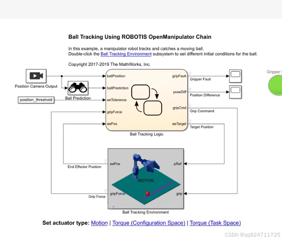
以下是一个基于MATLAB的机器人控制系统仿真模型代码示例。这个示例将包括运动学、动力学仿真、轨迹规划和简单的避障算法。为了便于理解，我们将使用一个两连杆机械臂作为示例。

---

1. 运动学仿真

运动学部分主要涉及正运动学（Forward Kinematics）和逆运动学（Inverse Kinematics）。

% 正运动学函数
function [x, y] = forward_kinematics(theta1, theta2, L1, L2)
    % 输入：关节角度 theta1, theta2 和连杆长度 L1, L2
    % 输出：末端执行器位置 (x, y)
    x = L1 * cos(theta1) + L2 * cos(theta1 + theta2);
    y = L1 * sin(theta1) + L2 * sin(theta1 + theta2);
end

% 逆运动学函数
function [theta1, theta2] = inverse_kinematics(x, y, L1, L2)
    % 输入：末端执行器位置 (x, y) 和连杆长度 L1, L2
    % 输出：关节角度 theta1, theta2
    c2 = (x^2 + y^2 - L1^2 - L2^2) / (2 * L1 * L2);
    s2 = sqrt(1 - c2^2); % 假设取正解
    theta2 = atan2(s2, c2);
    k1 = L1 + L2 * cos(theta2);
    k2 = L2 * sin(theta2);
    theta1 = atan2(y, x) - atan2(k2, k1);
end

---

2. 动力学仿真

动力学部分可以使用拉格朗日方程来建模。以下是两连杆机械臂的动力学方程实现。

function [ddq1, ddq2] = dynamics(theta1, theta2, dtheta1, dtheta2, L1, L2, m1, m2, g)
    % 输入：关节角度、角速度、连杆长度、质量、重力加速度
    % 输出：关节角加速度 ddq1, ddq2
    
    % 动力学参数
    I1 = (1/3) * m1 * L1^2; % 连杆1的转动惯量
    I2 = (1/3) * m2 * L2^2; % 连杆2的转动惯量
    
    % 拉格朗日方程计算
    M11 = I1 + I2 + m2 * L1^2 + 2 * m2 * L1 * L2 * cos(theta2);
    M12 = I2 + m2 * L1 * L2 * cos(theta2);
    M21 = M12;
    M22 = I2;
    
    C1 = -m2 * L1 * L2 * sin(theta2) * (2 * dtheta1 * dtheta2 + dtheta2^2);
    C2 = m2 * L1 * L2 * sin(theta2) * dtheta1^2;
    
    G1 = (m1 + m2) * g * L1 * cos(theta1) + m2 * g * L2 * cos(theta1 + theta2);
    G2 = m2 * g * L2 * cos(theta1 + theta2);
    
    % 矩阵形式求解
    M = [M11, M12; M21, M22];
    C = [C1; C2];
    G = [G1; G2];
    
    % 假设无外力输入
    tau = [0; 0]; % 关节力矩
    ddq = M \ (tau - C - G);
    ddq1 = ddq(1);
    ddq2 = ddq(2);
end

---

3. 轨迹规划

轨迹规划可以使用五次多项式插值来生成平滑的关节轨迹。

function [theta, dtheta, ddtheta] = trajectory_planning(t, t_start, t_end, theta_start, theta_end)
    % 输入：时间 t, 起始时间 t_start, 结束时间 t_end, 起始角度 theta_start, 结束角度 theta_end
    % 输出：关节角度 theta, 角速度 dtheta, 角加速度 ddtheta
    
    if t < t_start
        theta = theta_start;
        dtheta = 0;
        ddtheta = 0;
    elseif t > t_end
        theta = theta_end;
        dtheta = 0;
        ddtheta = 0;
    else
        T = t_end - t_start;
        a0 = theta_start;
        a1 = 0;
        a2 = 0;
        a3 = (10/T^3) * (theta_end - theta_start);
        a4 = (-15/T^4) * (theta_end - theta_start);
        a5 = (6/T^5) * (theta_end - theta_start);
        
        tau = t - t_start;
        theta = a0 + a1*tau + a2*tau^2 + a3*tau^3 + a4*tau^4 + a5*tau^5;
        dtheta = a1 + 2*a2*tau + 3*a3*tau^2 + 4*a4*tau^3 + 5*a5*tau^4;
        ddtheta = 2*a2 + 6*a3*tau + 12*a4*tau^2 + 20*a5*tau^3;
    end
end

---

4. 避障算法

简单的避障可以通过势场法实现。

function F_rep = obstacle_avoidance(x, y, obs_x, obs_y, obs_radius, repulsive_gain)
    % 输入：当前位置 (x, y)，障碍物位置 (obs_x, obs_y)，障碍物半径 obs_radius，排斥增益 repulsive_gain
    % 输出：排斥力 F_rep
    
    distance = sqrt((x - obs_x)^2 + (y - obs_y)^2);
    if distance <= obs_radius
        F_rep = repulsive_gain * (1/distance - 1/obs_radius) * ((x - obs_x)/distance, (y - obs_y)/distance);
    else
        F_rep = [0; 0];
    end
end

---

5. 完整仿真流程

将上述模块整合到一个仿真脚本中。

% 参数初始化
L1 = 1; L2 = 1; % 连杆长度
m1 = 1; m2 = 1; % 质量
g = 9.81; % 重力加速度
t_start = 0; t_end = 5; % 时间范围
theta1_start = 0; theta1_end = pi/4; % 关节1起始和结束角度
theta2_start = 0; theta2_end = pi/3; % 关节2起始和结束角度

% 障碍物参数
obs_x = 1.5; obs_y = 1.5; obs_radius = 0.5; repulsive_gain = 1;

% 仿真时间步长
dt = 0.01;
time = t_start:dt:t_end;

% 初始化变量
theta1 = zeros(size(time));
theta2 = zeros(size(time));

for i = 1:length(time)
    t = time(i);
    
    % 轨迹规划
    [theta1(i), ~, ~] = trajectory_planning(t, t_start, t_end, theta1_start, theta1_end);
    [theta2(i), ~, ~] = trajectory_planning(t, t_start, t_end, theta2_start, theta2_end);
    
    % 正运动学计算
    [x, y] = forward_kinematics(theta1(i), theta2(i), L1, L2);
    
    % 避障算法
    F_rep = obstacle_avoidance(x, y, obs_x, obs_y, obs_radius, repulsive_gain);
    
    % 动力学仿真
    [ddq1, ddq2] = dynamics(theta1(i), theta2(i), 0, 0, L1, L2, m1, m2, g);
end

% 绘图
figure;
plot(time, theta1, 'r', 'LineWidth', 1.5); hold on;
plot(time, theta2, 'b', 'LineWidth', 1.5);
xlabel('时间 (s)');
ylabel('关节角度 (rad)');
legend('关节1', '关节2');
title('关节角度随时间变化');
grid on;

---

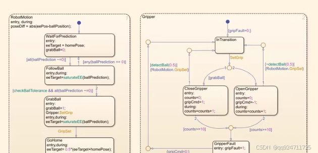
The diagram you’ve provided appears to be a state machine diagram for a robotic system, specifically focusing on the motion and gripping actions of a robot. This type of diagram is often used in robotics to define the states and transitions that control the behavior of the robot, such as moving towards a target, grabbing an object, and returning home.

Explanation of the Diagram

1. RobotMotion State Machine:

   • Entry: The initial state where the robot starts.
   • WaitForPrediction: The robot waits for a prediction about the ball’s position.
   • FollowBall: Once the prediction is received, the robot follows the ball.
   • GrabBall: The robot attempts to grab the ball.
   • GoHome: After grabbing the ball, the robot returns to its home position.

2. Gripper State Machine:

   • InTransition: The gripper is transitioning between states.
   • SetGrip: Setting the grip based on the command.
   • CloseGripper: The gripper closes to grab an object.
   • OpenGripper: The gripper opens to release an object.
   • GripperFault: Handling a fault condition if the gripper fails.

MATLAB Code Implementation

Below is a simplified MATLAB implementation of the state machines depicted in the diagrams. This code assumes you have functions to handle the transitions and actions within each state.

% Initialize variables
currentState = 'entry';
gripperState = 'inTransition';
ballPosition = [];
homePose = [0; 0; 0]; % Example home pose
eeTarget = homePose;
graspBall = false;
gripCmd = 0;
counts = 0;
grpfault = 0;

% Main loop
while true
    switch currentState
        case 'entry'
            poseDiff = abs(eePos - ballPosition);
            currentState = 'waitForPrediction';
            
        case 'waitForPrediction'
            if ~isempty(ballPrediction)
                eeTarget = homePose;
                graspBall = false;
                currentState = 'followBall';
                
            elseif any(isnan(ballPrediction))
                currentState = 'waitForPrediction';
                
            else
                currentState = 'waitForPrediction';
            end
            
        case 'followBall'
            eeTarget = saturateEE(ballPrediction);
            currentState = 'grabBall';
            
        case 'grabBall'
            if checkBallTolerance && all(ballPrediction > 0)
                currentState = 'goHome';
            else
                currentState = 'grabBall';
            end
            
        case 'goHome'
            eeTarget = 0.5 * (eeTarget + homePose);
            currentState = 'entry';
            
        otherwise
            currentState = 'entry';
    end
    
    switch gripperState
        case 'inTransition'
            if detectBall(0.5)
                gripperState = 'setGrip';
            elseif ~detectBall(0.5)
                gripperState = 'setGrip';
            end
            
        case 'setGrip'
            if graspBall
                gripperState = 'closeGripper';
            else
                gripperState = 'openGripper';
            end
            
        case 'closeGripper'
            counts = counts + 1;
            if counts >= 10
                currentState = 'grabBall';
                gripperState = 'inTransition';
            end
            
        case 'openGripper'
            counts = counts + 1;
            if counts >= 10
                currentState = 'waitForPrediction';
                gripperState = 'inTransition';
            end
            
        case 'gripperFault'
            grpfault = grpfault + 1;
            if grpfault >= 10
                currentState = 'entry';
                gripperState = 'inTransition';
            end
    end
    
    % Update eeTarget and other variables here
end

Notes:

• saturateEE: A function that saturates the end-effector target position.
• checkBallTolerance: A function that checks if the ball is within the tolerance.
• detectBall: A function that detects the ball.
• ballPrediction: An array or variable that holds the predicted ball position.
• eePos: The current end-effector position.
• eeTarget: The target end-effector position.
• graspBall: A boolean indicating whether the robot should grasp the ball.
• grpfault: A counter for gripper faults.

This code provides a basic framework for implementing the state machines shown in the diagrams. You would need to implement the specific functions (saturateEE, checkBallTolerance, detectBall, etc.) according to your application requirements.