机器学习：基于逻辑回归和高斯贝叶斯对人口普查数据集的分类与预测

• 机器学习：基于逻辑回归和高斯贝叶斯对人口普查数据集的分类与预测

作者：i阿极

作者简介：Python领域新星作者、多项比赛获奖者：博主个人首页

😊😊😊如果觉得文章不错或能帮助到你学习，可以点赞👍收藏📁评论📒+关注哦！👍👍👍

📜📜📜如果有小伙伴需要数据集和学习交流，文章下方有交流学习区！一起学习进步！💪

---

订阅专栏案例：机器学习
机器学习：基于逻辑回归对某银行客户违约预测分析
机器学习：学习k-近邻（KNN）模型建立、使用和评价
机器学习：基于支持向量机（SVM）进行人脸识别预测
决策树算法分析天气、周末和促销活动对销量的影响
机器学习：线性回归分析女性身高与体重之间的关系
机器学习：基于主成分分析（PCA）对数据降维
机器学习：基于朴素贝叶斯对花瓣花萼的宽度和长度分类预测
机器学习：学习KMeans算法，了解模型创建、使用模型及模型评价
机器学习：基于神经网络对用户评论情感分析预测
机器学习：朴素贝叶斯模型算法原理（含实战案例）
机器学习：逻辑回归模型算法原理（附案例实战）
机器学习：基于逻辑回归对优惠券使用情况预测分析
机器学习：基于逻辑回归对超市销售活动预测分析
机器学习：基于KNN对葡萄酒质量进行分类

---

---

1、数据说明

属性	数据类型	数值类型	字段描述
1	ID	-	String
2	age	Numeric	Integer
3	workclass	Categorical	String
4	fnlwgt	Continuous	Integer
5	education	Categorical	String
6	education_num	Numeric	Integer
7	marital_status	Categorical	String
8	occupation	Categorical	String
9	relationship	Categorical	String
10	race	Categorical	String
11	gender	Categorical	String
12	capital_gain	Numeric	Integer
13	capital_loss	Numeric	Integer
14	hours_per_week	Numeric	Integer
15	native_country	Categorical	String
16	income_bracket	Categorical	Integer

2、数据探索

导入模块

from plotly import __version__


import plotly.offline as offline
from plotly.offline import init_notebook_mode, iplot

init_notebook_mode(connected=True)
from plotly.graph_objs import *
import colorlover as cl
from plotly import tools
import pandas as pd
import numpy as np
colors = ['#e43620', '#f16d30','#d99a6c','#fed976', '#b3cb95', '#41bfb3','#229bac', 
'#256894', '#fed936', '#f36d30', '#b3cb25', '#f14d30','#49bfb5','#252bac',]

导入数据

data_train = pd.read_csv(r'/home/mw/income_census_train.csv')
data_test = pd.read_csv(r'/home/mw/income_census_test.csv')

数据集实例数与特征数，缺失值查看

print('原训练集shape:',data_train.shape)
print('原测试集shape:',data_test.shape)
print('原数据集实例数：',data_train.shape[0]+data_test.shape[0])

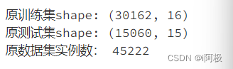
print('缺失值检测\n原训练集：',data_train.isnull().values.sum(), ',原测试集：',data_test.isnull().values.sum())

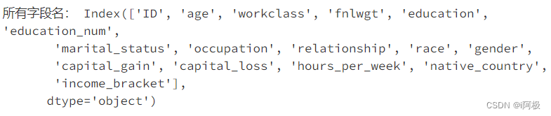
print('所有字段名：',data_train.columns)

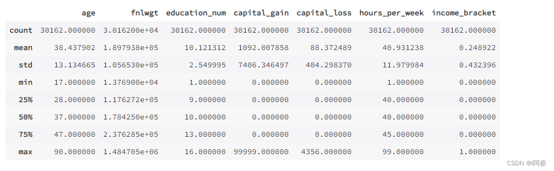
各个特征的描述与相关总结

data_train.describe()

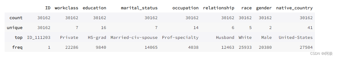
展示所有类型特征

data_train.describe(include=['O'])

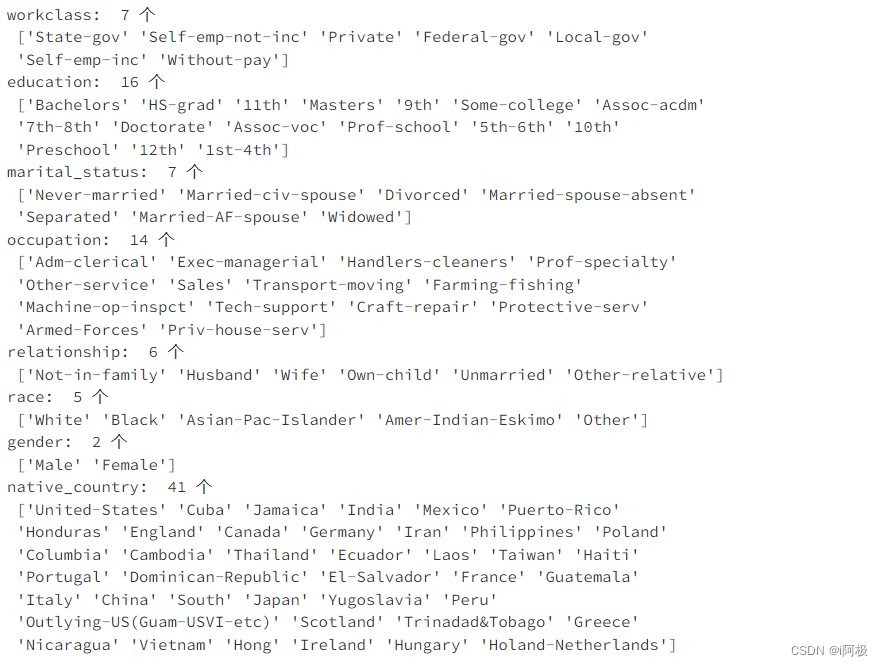
查看8个categorial数据类型的属性唯一值

print('workclass: ',len(data_train['workclass'].unique()),'个\n',data_train['workclass'].unique())
print('education: ',len(data_train['education'].unique()),'个\n',data_train['education'].unique())
print('marital_status: ',len(data_train['marital_status'].unique()),'个\n',data_train['marital_status'].unique())
print('occupation: ',len(data_train['occupation'].unique()),'个\n',data_train['occupation'].unique())
print('relationship: ',len(data_train['relationship'].unique()),'个\n',data_train['relationship'].unique())
print('race: ',len(data_train['race'].unique()),'个\n',data_train['race'].unique())
print('gender: ',len(data_train['gender'].unique()),'个\n',data_train['gender'].unique())
print('native_country: ',len(data_train['native_country'].unique()),'个\n',data_train['native_country'].unique())

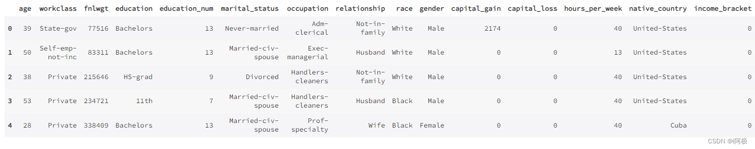
data = data_train.drop(['ID'],axis = 1)
data.head()

3、数据预处理

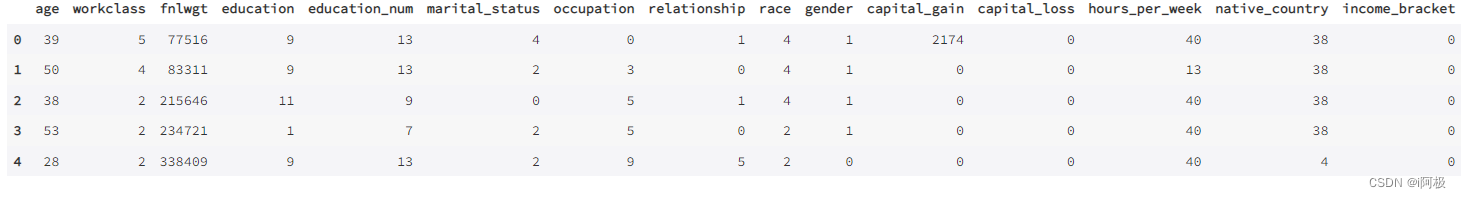
将oject数据转化为int类型

for feature in data.columns:
    if data[feature].dtype == 'object':
        data[feature] = pd.Categorical(data[feature]).codes # codes	这个分类的分类代码
data.head()

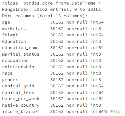
此时在查看数据每个字段的数值类型都是int类型。

data.info()

4、建立模型

选取特征数据与类别数据

from sklearn.preprocessing import StandardScaler
from sklearn.linear_model import LogisticRegression
from sklearn.model_selection import train_test_split
X_df = data.iloc[:,data.columns != 'income_bracket']
y_df = data.iloc[:,data.columns == 'income_bracket']
X = np.array(X_df)
y = np.array(y_df)

标准化数据

scaler = StandardScaler()
X = scaler.fit_transform(X)

5、特征选取（Feature Selection）

from sklearn.tree import DecisionTreeClassifier
# from sklearn.decomposition import PCA

# fit an Extra Tree model to the data
tree = DecisionTreeClassifier(random_state=0)
tree.fit(X, y)

# 显示每个属性的相对重要性得分
relval = tree.feature_importances_

trace = Bar(x = X_df.columns.tolist(), y = relval, text = [round(i,2) for i in relval], textposition= "outside", marker = dict(color = colors))
iplot(Figure(data = [trace], layout = Layout(title="特征重要性", width = 800, height = 400, yaxis = dict(range = [0,0.25]))))

from sklearn.feature_selection import RFE

# 使用决策树作为模型
lr = DecisionTreeClassifier()
names = X_df.columns.tolist()

# 将所有特征排序
selector = RFE(lr, n_features_to_select = 10)
selector.fit(X,y.ravel())

print("排序后的特征：",sorted(zip(map(lambda x:round(x,4), selector.ranking_), names)))

# 得到新的dataframe
X_df_new = X_df.iloc[:, selector.get_support(indices = False)]
X_df_new.columns

X_new = scaler.fit_transform(np.array(X_df_new)) # 数组化 + 标准化
X_train, X_test, y_train, y_test = train_test_split(X_new,y) # 切分

from sklearn.linear_model import LogisticRegression
from sklearn.naive_bayes import GaussianNB
from sklearn import metrics
from sklearn.metrics import confusion_matrix,roc_curve, auc, recall_score, classification_report

import matplotlib.pyplot as plt

import itertools

# 绘制混淆矩阵
def plot_confusion_matrix(cm, classes,
                          title='Confusion matrix',
                          cmap=plt.cm.Blues):
    """
    This function prints and plots the confusion matrix.
    Normalization can be applied by setting `normalize=True`.
    """
    plt.imshow(cm, interpolation='nearest', cmap=cmap)
    plt.title(title)
    plt.colorbar()
    tick_marks = np.arange(len(classes))
    plt.xticks(tick_marks, classes, rotation=0)
    plt.yticks(tick_marks, classes)

    thresh = cm.max() / 2.
    for i, j in itertools.product(range(cm.shape[0]), range(cm.shape[1])):
        plt.text(j, i, cm[i, j],
                 horizontalalignment="center",
                 color="white" if cm[i, j] > thresh else "black")

    plt.tight_layout()
    plt.ylabel('True label')
    plt.xlabel('Predicted label')

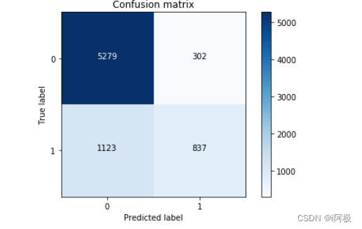
6、逻辑回归（Logistic Regression）

# instance
lr = LogisticRegression()
# fit
lr_clf = lr.fit(X_train,y_train.ravel())
# predict
y_pred = lr_clf.predict(X_test)

print('LogisticRegression %s' % metrics.accuracy_score(y_test, y_pred))

cm = confusion_matrix(y_test, y_pred)

class_names = [0,1]
plt.figure()
plot_confusion_matrix(cm , classes=class_names, title='Confusion matrix')
plt.show()

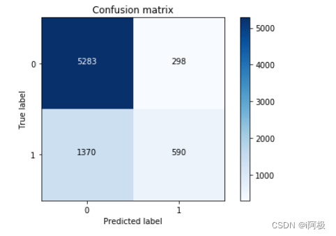
7、高斯贝叶斯（Gaussian Naive Bayes）

gnb = GaussianNB()
gnb_clf = gnb.fit(X_train, y_train.ravel())
y_pred2 = gnb_clf.predict(X_test)

print('GaussianNB %s' % metrics.accuracy_score(y_test, y_pred2))

cm = confusion_matrix(y_test, y_pred2)

class_names = [0,1]
plt.figure()
plot_confusion_matrix(cm , classes=class_names, title='Confusion matrix')
plt.show()

---

📢文章下方有交流学习区！一起学习进步！💪💪💪
📢首发CSDN博客，创作不易，如果觉得文章不错，可以点赞👍收藏📁评论📒
📢你的支持和鼓励是我创作的动力❗❗❗