神经网络——Tensor、计算图、训练方法

Tensor、Variable 和 Parameter

经过 Pytorch 0.4.0 的更新后，前两个都是一个 torch.Tensor 对象，可以理解为两者等价；后者是 Parameter 对象。

Tensor 包含如下属性：

• data，该 tensor 的值。
• required_grad，该 tensor 是否连接在计算图（computational graph）上。
• grad，如果 required_grad 是 True，则这个属性存储了反向传播时该 tensor 积累的梯度（这个梯度也是一个 tensor）。
• grad_fn，该 tensor 计算梯度的函数。
• is_leaf，在计算图中两种情况下 is_leaf 是 True：模型需要更新的参数 W 和模型的输入 x。is_leaf 和 required_grad 都是 True，该 tensor 才会将计算图中的梯度积累到 grad 属性中。

Parameter 与 Tensor 相比，多了两个特性：

• 与 model 融为一体，当使用 model.cuda() 时 model 中所有的 Parameter 都会装载到 cuda 上。
• 可以被 model.parameters 枚举出来，这样结合 optimizer 可以实现参数的更新。

计算图

前向计算时构建计算图，梯度是反向传播时计算，为了节省显存反向传播完计算图被释放。以 c = a*b 为例：

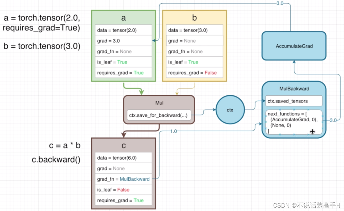
b 的 requires_grad 是 False，所以梯度计算时 b 是常数3，因此只计算梯度到 a 的 grad。

反向传播时 c.backward() 调用 MulBackward 来计算 a 和 b 的梯度：

前向计算和反向传播代码以 Swish 激活函数为例：

​class Swish(torch.autograd.Function):

    @staticmethod
    def forward(ctx, i):
        result = i * torch.sigmoid(i)
        ctx.save_for_backward(i)
        return result
    @staticmethod
    def backward(ctx, grad_output):
        i = ctx.saved_variables[0]
        sigmoid_i = torch.sigmoid(i)
        return grad_output * (sigmoid_i * (1 + i * (1 - sigmoid_i)))

class Swish_module(nn.Module):
    def forward(self, x):
        return Swish.apply(x)

训练方法

神经网络训练时有两部分会占用 GPU 的显存，第一部分是模型的参数权重；第二部分是输入模型的数据进行 forward 时，经过每一个神经元时算出的存储在计算图中的 activation（上面 Swish 代码中的 ctx.save_for_backward(i)？）。

常见的节省显存的训练方法有 Gradient Checkpointing 和混合精度训练。

Gradient Checkpointing

出自2016年的论文《Training Deep Nets With Sublinear Memory Cost》，论文证明这种方法能将模型的空间复杂度从 O(n) 降低到 O(sqrt(n))。简单来说，gradient checkpointing 会忽略一些 activation 来减少计算图占用的显存，在反向传播时重新计算 activation。当然这样做会减慢训练速度，这是一种 compute time 和 memory 的 trade-off。

前向计算时不用存储 activation，之后到每一个模块的反向传播中重新计算 activation，反向传完即释放显存。这时占用显总共需要的显存是每个模块需要的显存的最大值，而不是这些值的加和，这样就达到了节省显存的目的。

During the forward pass, PyTorch saves the input tuple to each function in the model. During backpropagation, the combination of input tuple and function is recalculated for each function in a just-in-time manner, plugged into the gradient formula for each function that needs it, and then discarded.

Pytorch 中提供了 torch.utils.checkpoint.checkpoint 和 torch.utils.checkpoint.checkpoint_sequential 来实现 gradient checkpointing。

torch.utils.checkpoint.checkpoint

class CIFAR10Model(nn.Module):
    def __init__(self):
        super().__init__()
        self.cnn_block_1 = nn.Sequential(*[nn.Conv2d(3, 32, 3, padding=1), nn.ReLU(), nn.Conv2d(32, 64, 3, padding=1), nn.ReLU(), nn.MaxPool2d(kernel_size=2), nn.Dropout(0.25)])
        self.cnn_block_2 = nn.Sequential(*[nn.Conv2d(64, 64, 3, padding=1), nn.ReLU(), nn.Conv2d(64, 64, 3, padding=1), nn.ReLU(), nn.MaxPool2d(kernel_size=2), nn.Dropout(0.25)])
        self.flatten = lambda inp: torch.flatten(inp, 1)
        self.head = nn.Sequential(*[nn.Linear(64 * 8 * 8, 512), nn.ReLU(), nn.Dropout(0.5), nn.Linear(512, 10)])
    
    def forward(self, X):
        X = self.cnn_block_1(X)
        X = self.cnn_block_2(X)
        X = self.flatten(X)
        X = self.head(X)
        return X

加上 checkpointing：

class CIFAR10Model(nn.Module):
    def __init__(self):
        super().__init__()
        self.cnn_block_1 = nn.Sequential(*[nn.Conv2d(3, 32, 3, padding=1), nn.ReLU(), nn.Conv2d(32, 64, 3, padding=1), nn.ReLU(), nn.MaxPool2d(kernel_size=2)], nn.Dropout(0.25))
        self.cnn_block_2 = nn.Sequential(*[nn.Conv2d(64, 64, 3, padding=1), nn.ReLU(), nn.Conv2d(64, 64, 3, padding=1), nn.ReLU(), nn.MaxPool2d(kernel_size=2)])
        self.dropout_2 = nn.Dropout(0.25)
        self.flatten = lambda inp: torch.flatten(inp, 1)
        self.linearize = nn.Sequential(*[ nn.Linear(64 * 8 * 8, 512), nn.ReLU()])
        self.dropout_3 = nn.Dropout(0.5)
        self.out = nn.Linear(512, 10)
    
    def forward(self, X):
        X = self.cnn_block_1(X)
        X = torch.utils.checkpoint.checkpoint(self.cnn_block_2, X)
        X = self.dropout_2(X)
        X = self.flatten(X)
        X = self.linearize(X)
        X = self.dropout_3(X)
        X = self.out(X)
        return X

需要注意 Dropout 和 BN 层。

因为需要进行两次前向计算，每一个 Dropout 激活的神经元位置是不同的，这样就会导致错误。应该将 gradient checkpointing 放在 Dropout 层之前或之后；

而 BN 层则会在两次前向计算中和 momentum 参数一起更新两次均值和方差 ，可以通过将 momentum 设置为 sqrt(momentum) 来修正，均值不变的话方差就不会变：

original_rm, original_nm = running_mean, new_mean

# Originally, we have a running_mean to start from
momemtum = 0.9
# running mean after the first forward pass. We want to match this 
# when we use checkpointing
running_mean1 = original_nm * 0.1 + original_rm * 0.9

# With checkpointing, we use momentum = sqrt(0.9) and make two passes
momentum = sqrt(0.9)
runing_mean = original_nm * (1 - sqrt(0.9)) + original_rm * sqrt(0.9)      # Eq (1) 
# Note that in the second forward pass, since the inputs are same, the 
# new_mean value doesn't change
running_mean2 = original_nm * (1 - sqrt(0.9)) + running_mean * sqrt(0.9)   # Eq (2) 

#Substitue value of running_mean from Eq(1) to Eq(2)
assert running_mean2 == running_mean1

同时需要注意的是只将第二个 cnn_block 放入了 checkpoint，因为 checkpoint 会根据输入数据是否需要更新来决定 checkpoint 中的参数是否进行更新。而最开始的 X 是原始数据，显然不需要更新，所以如果将原始数据也放入 checkpoint 的话，会导致之后的 checkpoint 里参数都不更新，也就是模型没有从数据中学习。

checkpoint 的实现如下，可以看到与上面 Swish 在 forward 内的区别是 outputs 之前加上了 with torch.no_grad：

class CheckpointFunction(torch.autograd.Function):

    @staticmethod
    def forward(ctx, run_function, preserve_rng_state, *args):
        check_backward_validity(args)
        ctx.run_function = run_function
        ctx.preserve_rng_state = preserve_rng_state
        if preserve_rng_state:
            ctx.fwd_cpu_state = torch.get_rng_state()
            # Don't eagerly initialize the cuda context by accident.
            # (If the user intends that the context is initialized later, within their run_function, we SHOULD actually stash the cuda state here. 
            # Unfortunately, we have no way to anticipate this will happen before we run the function.)
            ctx.had_cuda_in_fwd = False
            if torch.cuda._initialized:
                ctx.had_cuda_in_fwd = True
                ctx.fwd_gpu_devices, ctx.fwd_gpu_states = get_device_states(*args)
        ctx.save_for_backward(*args)
        with torch.no_grad():
            outputs = run_function(*args)
        return outputs

    @staticmethod
    def backward(ctx, *args):
        if not torch.autograd._is_checkpoint_valid():
            raise RuntimeError("Checkpointing is not compatible with .grad(), please use .backward() if possible")
        inputs = ctx.saved_tensors
        # Stash the surrounding rng state, and mimic the state that was present at this time during forward.  
        # Restore the surrouding state when we're done.
        rng_devices = []
        if ctx.preserve_rng_state and ctx.had_cuda_in_fwd:
            rng_devices = ctx.fwd_gpu_devices
        with torch.random.fork_rng(devices=rng_devices, enabled=ctx.preserve_rng_state):
            if ctx.preserve_rng_state:
                torch.set_rng_state(ctx.fwd_cpu_state)
                if ctx.had_cuda_in_fwd:
                    set_device_states(ctx.fwd_gpu_devices, ctx.fwd_gpu_states)
            detached_inputs = detach_variable(inputs)
            with torch.enable_grad():
                outputs = ctx.run_function(*detached_inputs)

        if isinstance(outputs, torch.Tensor):
            outputs = (outputs,)
        torch.autograd.backward(outputs, args)
        grads = tuple(inp.grad if isinstance(inp, torch.Tensor) else inp for inp in detached_inputs)
        return (None, None) + grads

torch.utils.checkpoint.checkpoint_sequential

比 checkpoint 要麻烦一些，需要自己设定将 model 分成几个 segment。checkpoint_sequential 会将 model 分成不同的 segment，不在前向传播时计算这些 segment 的 activation（对应 Swish 代码中的 result = i * torch.sigmoid(i)？）。在反向传播时，这些 segment 的 activation 才被计算出来，这时总共需要的显存是每个 segment 需要占用的显存中最大的那一个，而不是这些的加和。

import torch
import torch.nn as nn
from torch.utils.checkpoint import checkpoint_sequential

# a trivial model
model = nn.Sequential(nn.Linear(100, 50), nn.ReLU(), nn.Linear(50, 20), nn.ReLU(), nn.Linear(20, 5), nn.ReLU())
# model input
input_var = torch.randn(1, 100, requires_grad=True)
# the number of segments to divide the model into
segments = 2
# get the modules in teh model, should be in order
modules = [module for k, module in model.modulles.items()]
# finally, apply checkpointing to the model, note the code that this replaces:
# out = model(input_var)
out = checkpoint_sequential(modules, segments, input_var)
# backpropagate
out.sum().backwards()

pytorch_memonger/Checkpointing_for_PyTorch_models.ipynb at master · prigoyal/pytorch_memonger · GitHub
Training larger-than-memory PyTorch models using gradient checkpointing
Explore Gradient-Checkpointing in PyTorch

混合精度训练

Apex 和 amp

Apex：全称 A Pytorch Extension，一种 Pytorch 的扩展插件，目的是为了用户能够快速实现 amp。

amp（auto mixed precision）：自动半精度，是单精度 float 和半精度 float16 的混合，出自论文《MIXED PRECISION TRAINING》。

优点

与单精度 float（32 bit，4个字节）相比，半精度 float16 仅有 16bit，2个字节组成，需要的存储空间是 float 的一半。显存占用更少，训练的时候可以使用更大的 batchsize；

训练速度更快，因为在 NVIDIA 比较新版本的 GPU 上都搭载了 tensor core。tensor core 是专门为这种操作设计：将两个 fp16 的矩阵相乘，再将结果加在一个 fp16 或 fp32 的矩阵上。模型进行前向计算、反向传播以及参数更新时，都会用到乘法和加法的运算。

tensor core 和 CUDA core 的区别可以简单理解为：前者每个 GPU 时钟执行一次矩阵乘法，后者每个 GPU 时钟执行一次值乘法。

缺点

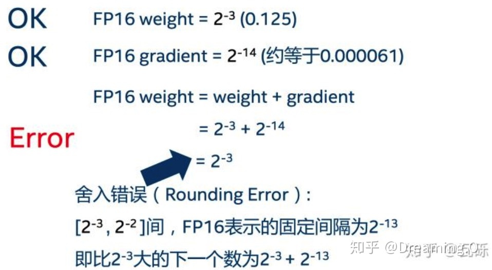
溢出错误。float16 最大范围是 [-65504，-66504]，float16 能表示的精度范围是2的-24次方，超过这个数值的数字会被直接置0。对于深度学习而言，最大的问题在于 Underflow（下溢出）。在训练后期，例如激活函数的梯度会非常小， 甚至在梯度乘以学习率后，值会更加小。

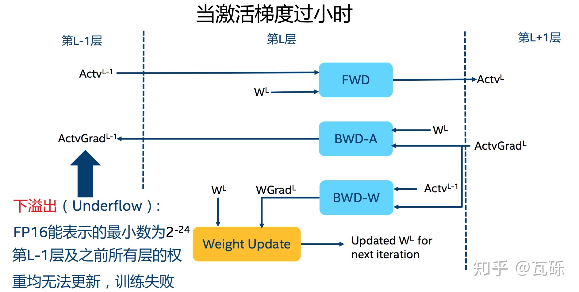
舍入误差。当梯度过小，小于当前区间内的最小间隔时，该次梯度更新可能会失败。

解决办法

对于这两个缺点的解决办法：混合精度训练+动态损失放大。

混合精度训练。对 weights、activations、gradients 等在前向计算和反向传播时适合采用 fp16 的操作，其存储和计算都使用 fp16，其余的用 fp32 进行计算，计算之后依然采用 fp16 进行存储，同时拷贝一份 fp32 的 weights 用于参数更新。

在论文中还提到一个『计算精度』的问题：在某些模型中，fp16 矩阵乘法的过程中，需要利用 fp32 来进行矩阵乘法中间的累加（accumulated），然后再将 fp32 的值转化为 fp16 进行存储。 换句不太严谨的话来说，也就是利用 fp16 进行乘法和存储，利用 fp32 来进行加法计算。 这么做的原因主要是为了减少加法过程中的舍入误差，保证精度不损失。

pytorch混合精度训练_cdknight_happy的博客-CSDN博客_scaler.unscale_​​​

（受不了 CSDN 的水印🤬🤬🤬）

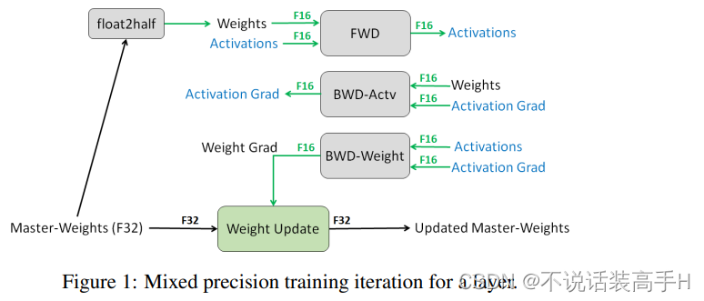
在参数更新时，其公式为：权重 = 旧权重 + lr * 梯度，而在深度模型中 lr * 梯度 这个值往往是非常小的。如果也使用 fp16 来进行相加的话， 则很可能会出现上面所说的 舍入误差 这个问题，导致更新无效，所以需要拷贝一份 fp32 的 weights。

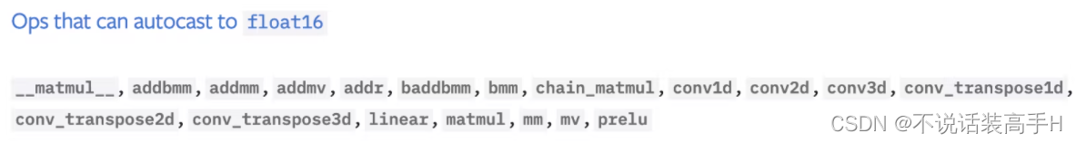
适合采用 fp16 的一些操作：

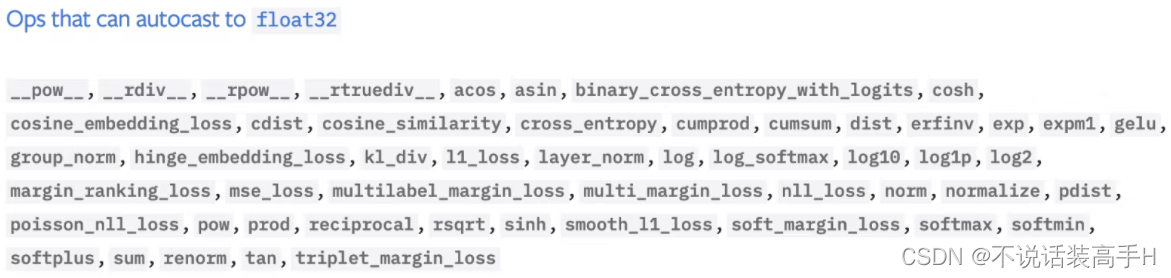
适合采用 fp32 的一些操作：

动态损失放大（Loss Scale）。是为了解决 溢出错误，训练到了后期梯度（特别是激活函数平滑段的梯度）会特别小，fp16 表示容易产生下溢现象。为了解决梯度过小的问题，对计算出来的 loss 值进行 scale。

由于链式法则的存在，loss 上的 scale 也会作用在梯度上，这样比起对每个梯度进行 scale 更加划算。

scale 过后的梯度，就会平移到 fp16 有效的展示范围内。这样，scaled-gradient 就可以一直使用 fp16 进行存储了。只有在进行更新的时候，才会将 scaled-gradient 转化为 fp32，同时将 scale 抹去。

混合精度训练的两种方式

NVIDIA apex

from apex import amp
model, optimizer = amp.initialize(model, optimizer, opt_level="O1") # 这里是“欧一”，不是“零一”
with amp.scale_loss(loss, optimizer) as scaled_loss:
    scaled_loss.backward()#梯度自动缩放
optimizer.step()

其中只有一个 opt_level 需要用户自行配置：

• o0：纯FP32训练，可以作为 accuracy 的 baseline；
• o1：混合精度训练（推荐使用），根据黑白名单自动决定使用 fp16（GEMM，卷积）还是 fp32（Softmax）进行计算。
• o2：几乎都是 fp16混合精度训练，不存在黑白名单，除了 Batch norm，几乎都是用 fp16 计算。
• o3：纯 fp16 训练，很不稳定，但是可以作为 speed 的 baseline；

torch 原生支持的amp

from torch.cuda.amp import autocast as autocast, GradScaler

scaler = GradScaler()

        ...
        # 前向过程为 model 和 loss 开启 autocast
        with autocast():
            output = model(input)
            loss = loss_fn(output, target)
        # Scales loss，这是因为半精度的数值范围有限，因此需要用它放大
        scaler.scale(loss).backward()
        # unscale之前放大后的梯度，但是scale太多可能出现inf或NaN，故其会判断是否出现了inf/NaN
        # 如果梯度的值不是 infs 或者 NaNs, 那么调用optimizer.step()来更新权重,
        # 如果检测到出现了inf或者NaN，就跳过这次梯度更新，同时动态调整scaler的大小
        scaler.step(optimizer)
        # 查看是否要更新scaler,这个要注意不能丢
        scaler.update()

每个模型 scale 的程度是不确定的，同时训练前期的梯度比训练后期的梯度要大得多。如果 scale 不合适的话，又可能导致 Overflow。

PyTorch 使用 exponential backoff 来解决这个问题，scale 在刚开始的时候为2的16次方（下面代码中的 init_scale=65536.0），之后每隔一段时间加倍，直到梯度上溢出现 inf（scaler.scale(loss).backward() 检查是否上溢）。此时这个 batch 不更新参数（scaler.step(optimizer) 抛弃这个 batch，不更新参数），将 scale 减半。这里的 scale 用 GradScaler() 实现，这些参数都是默认的：

torch.cuda.amp.GradScaler(
    init_scale=65536.0, growth_factor=2.0, backoff_factor=0.5,
    growth_interval=2000, enabled=True
)

pytorch原生支持的apex混合精度和nvidia apex混合精度AMP技术加速模型训练效果对比_colourmind的博客-CSDN博客_apex.amp
【PyTorch】唯快不破：基于Apex的混合精度加速 - 知乎
A developer-friendly guide to mixed precision training with PyTorch
浅谈混合精度训练 - 知乎 

Dsitributed training

分为 Data parallelization 和 Model parallelization。前者的做法是为每个 GPU 分配当前 model 的副本和当前 batch data 的一个 slice（DP），每个 GPU 独立完成前向计算和反向传播，计算出梯度后将各 GPU 的梯度相加求平均，用平均的梯度更新参数（DP）。后者是为每个 GPU 分配当前 model 的一个 slice，也就是其中的一些层。

前者更容易实现，因为不需要解剖模型结构，这里主要关注前者，API 为 DistributedDataParalled（DDP） 和 DataParallel（DP）。

先说区别：

• DataParallel 采用单进程多线程的方法实现（所以由于 GIL 锁的限制，性能不如 DistributedDataParalled），参数更新算法采用 Parameter Server，只能在单机上用，不支持混合精度训练；
• DistributedDataParalled 采用多进程的方法实现，参数更新算法采用 Ring AllReduce，可以在多机上用，支持混合精度训练，需要注意 BN 层的数据同步。

参数更新算法

常用的两种参数同步的算法：Parameter Server 和 Ring AllReduce。假设有5张 GPU：

• Parameter Server

需要将一个 GPU 设置为 Reducer，Reducer 将 data batch 分成五份分到各个卡上，每张卡负责自己的那一份 slice 的训练（有效 batch size = batch size）。反向传播得到梯度返回给 Reducer 上做累积，更新完权重后再分发给各个卡。

缺点是有很严重的木桶效应；负载不均衡，Reducer 需要额外的显存空间来存储各个 GPU 的梯度。

• Ring AllReduce

5张卡以环形相连，每张卡都有一份模型的副本和整个 batch size（有效 batch size = batch size*5）。每张卡都有左手卡和右手卡，一个负责接收，一个负责发送，循环4次完成梯度累积（Scatter Reduce），再循环4次做参数同步（All Gather）。

Scatter Reduce 步骤中，GPU 将交换数据，使每个 GPU 都得到最终结果的一个块。这个步骤与梯度的反向传播一同进行，来缓解通信时的 bottleneck。

在 All Gather 步骤中，各 GPU 将交换这些块，以便所有 GPU 得到完整的最终结果。

Each GPU does its own forward pass, and then the gradients are all-reduced across the GPUs. Gradients for each layer do not depend on previous layers, so the gradient all-reduce is calculated concurrently with the backwards pass to futher alleviate the networking bottleneck. At the end of the backwards pass, every node has the averaged gradients, ensuring that the model weights stay synchronized.

分布式训练 — 理论基础_love1005lin的博客-CSDN博客_分布式训练

Distributed data parallel training using Pytorch on AWS | Telesens

DistributedDataParalled

有三种不同的实现：Open MPI，NVIDIA NCCL 和 Facebook Gloo。

下面介绍的方法只能用在单机多卡的情况下，假设有4块 GPU：

根据官网的介绍，如果使用 CPU 进行分布式计算，建议使用 Gloo，如果使用 GPU 进行分布式计算，建议使用 NCCL，不推荐多 GPU 时使用 MPI。这些都是 dist.init_process_group() 的第一个 backend（后端）参数可以用的方法。

进程初始化。先看代码：

import torch
import torch.distributed as dist
import torch.multiprocessing as mp

def init_process(rank, size, backend='gloo'):
    """ Initialize the distributed environment. """
    os.environ['MASTER_ADDR'] = '127.0.0.1'
    os.environ['MASTER_PORT'] = '29500'
    dist.init_process_group(backend, rank=rank, world_size=size) # init_method 默认为 “env://”

def train(rank, num_epochs, world_size):
    init_process(rank, world_size)
    print(
        f"Rank {rank + 1}/{world_size} process initialized.\n"
    )
    # rest of the training script goes here!

WORLD_SIZE = torch.cuda.device_count()
if __name__=="__main__":
    mp.spawn(
        train, args=(NUM_EPOCHS, WORLD_SIZE),
        nprocs=WORLD_SIZE, join=True
    )

world_size 是进程数，rank 是当前进程的顺序数。torch.cuda.device_count() 会统计出当前所有可用的 GPU 数为4，所以 mp.spawn 会引出4个不同的进程，默认情况下 rank0 是主进程。

dist.init_process_group() 用于初始化进程及 GPU 通信方式（Gloo）和参数的获取方式（“env：//” 表示通过环境变量），建立进程间的通信，当完成该函数时进程被销毁。

os.environ['MASTER_PORT'] = '29500'  是进程间通信的端口，os.environ['MASTER_ADDR'] = '127.0.0.1' 是多机间通信的 IP，这两个均是通过环境变量设置的。

多机多卡间的通信要复杂一些，除了设置端口外还需要设置 IP 地址。

数据/ IO 操作。任何数据下载和 IO 的操作都必须隔离在主进程上：

def tarin( ...):
    ...
    if rank == 0:
        downloading_dataset()
        downloading_model_weights()
    dist.barrier()
    print(
        f"Rank {rank + 1}/{world_size} training process passed data download barrier.\n"
    )

在完成下载操作前，dist.barrier() 阻止其他进程继续向下执行。我们需要保证每张 GPU 上分到的都是不同的数据，这里需要用到 DistributedSampler。rank 和 num_replicas 参数也可以不设置，源码中会自动获取。

dataset = PascalVOCSegmentationDataset()
sampler = DistributedSampler(
    dataset, rank=rank, num_replicas=world_size, shuffle=True
)
dataloader = DataLoader(
    dataset, batch_size=8, sampler=sampler
)

之后将 DistributedSampler 送到 DataLoader 里，此时有效的 batch size 是4*8=32。

当需要保存模型的参数时，也需要主进程来完成：

if rank == 0:
    if not os.path.exists('/spell/checkpoints/'):
        os.mkdir('/spell/checkpoints/')
        torch.save(
            model.state_dict(),
            f'/spell/checkpoints/model_{epoch}.pth'
        )

将 tensor 移至 GPU。代码如下：

def train( ...):
    ...
    model.cuda(rank)
    for i, (batch, target) in enumerate(dataloader):
        batch = batch.cuda(rank)
        target = target.cuda(rank)

固定种子。每个进程上的种子应该是相同的，否则会计算出错误的梯度导致不能收敛。

seed = 1234
np.random.seed(seed)
random.seed(seed)
torch.manual_seed(seed)
torch.set_rng_state(torch.manual_seed(seed).get_state())
torch.cuda.manual_seed_all(seed)
torch.backends.cudnn.deterministic = True
torch.backends.cudnn.benchmark = False

完成上述步骤后，我们就可以调用 DistributedDataParalled 来进行单机多卡训练：

model = DistributedDataParallel(model, device_ids=[rank])

同步 BN。统计多卡数据上的均值和方差，来获得更好的估计。

model = torch.nn.SyncBatchNorm.convert_sync_batchnorm(model)

因为用了 mp.spawn()，所以可以在命令行直接使用 python .py 来执行程序。

总结一下，DistributedDataParalled 的步骤为：

• 固定种子，设置通信端口和 IP，使用 torch.distributed.init_process_group() 初始化进程组。
• 使用 torch.utils.data.distributed.DistributedSampler() 创建 DataLoader。
• 使用 torch.nn.parallel.DistributedDataParallel() 创建分布式模型，同步 BN。
• 使用 torch.distributed.launch /直接 python .py 开始训练。

没有用 mp.spawn() 的话，就需要 python -m torch.distributed.launch 的方法来启动训练：分布式训练 - 单机多卡（DP和DDP）_love1005lin的博客-CSDN博客_单机多卡

DataParallel

只需要一行代码：

model = nn.DataParallel(model.to(device), device_ids=gpus, output_device=gpus[0])

• divice_ids：参与训练的 GPU，不设置将默认采用所有 GPU。
• output_device：用于汇总梯度的 GPU 是哪个，默认为 GPU0。

import torch
import torch.distributed as dist

gpus = [0, 1, 2, 3]
torch.cuda.set_device('cuda:{}'.format(gpus[0]))

train_dataset = ...

train_loader = torch.utils.data.DataLoader(train_dataset, batch_size=...)

model = ...
model = nn.DataParallel(model.to(device), device_ids=gpus, output_device=gpus[0])

optimizer = optim.SGD(model.parameters())

for epoch in range(100):
   for batch_idx, (data, target) in enumerate(train_loader):
      images = images.cuda(non_blocking=True)
      target = target.cuda(non_blocking=True)
      ...
      output = model(images)
      loss = criterion(output, target)
      ...
      optimizer.zero_grad()
      loss.backward()
      optimizer.step()

Distributed model training in PyTorch using DistributedDataParallel

多机多卡

分布式训练 - 多机多卡 (DDP)_love1005lin的博客-CSDN博客_nproc_per_node

Distributed data parallel training in Pytorch