7月28日深度学习笔记——GAN

---

前言

本文为7月28日深度学习笔记， 分为三个章节：

• Theory behind GAN：Generation、max V(G, D)、Algorithm；
• Framework of GAN：f-divergence、Fenchel Conjugate；
• Tips for Improving GAN：JS divergence is not suitable、Least Square GAN（LSGAN）、Wasserstein GAN（WGAN）.

---

一、Theory behind GAN

1、Generation

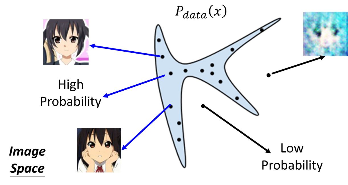
• $x$: an image(a high-dimensional vector) ；
• Find data distribution $P_{data}(x)$.
  

(1)、Maximum Likelihood Estimation = Minimize KL Divergence

• Given $P_{data}(x)$(sample from it);
• We have a distribution $P_G(x;\theta )$:
  • we want to find $\theta$ such that $P_G(x;\theta )$ close to $P_{data}(x)$;
• Sample { x 1 , x 2 , … , x m } \{x^1, x^2, …, x^m \} {x1,x2,…,xm} from $P_{data}(x)$;
  • we can compute $P_G(x^i;\theta )$
  • Likelihood of generating the samples:
    $$L=\prod _{i=1}^m{P}_G(x^i;\theta )$$
  • Find ${\theta }^{\ast }$ maximizing the likelihood.
    $${\theta }^{\ast }=argmax\prod _{i=1}^m{P}_G(x^i;\theta )=argmaxlog\prod _{i=1}^m{P}_G(x^i;\theta )=argmax\sum _{i=1}^{m}log{P}_G(x^i;\theta )\approx argmax{E}_{x{P}_{data}}[log{P}_G(x^i;\theta )]=argmax\underset{x}{\int }{P}_{data}(x)log{P}_G(x;\theta )dx-\underset{x}{\int }{P}_{data}(x)log{P}_{data}(x)dx=argminKL(P_{data}||P_G)$$

(2)、Generator

A generator $G$ is a network. The network defines a probability distribution $P_G$.

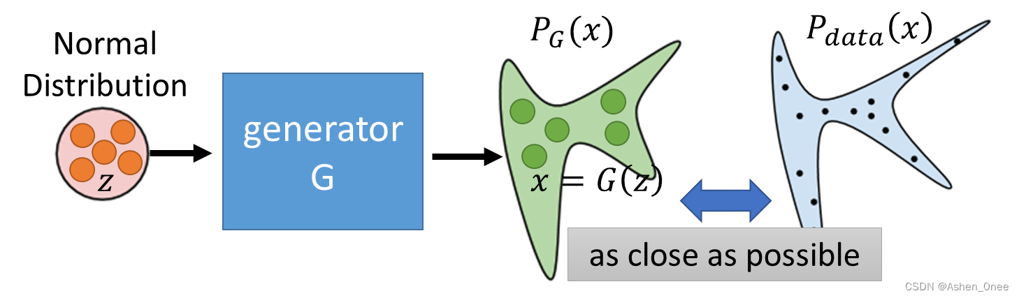
Divergence between distributions $P_G$ and $P_{data}$:
$$G^{\ast }=argminDiv(P_G,P_{data})$$

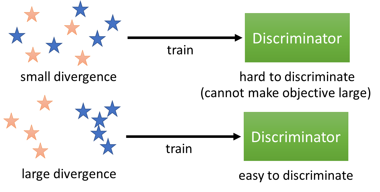
(3)、Discriminator

Objective Function for D:
$$V(G,D)=E_{x{P}_{data}}[logD(x)]+E_{x{P}_G}[log(1-D(x))]$$

Training:
$$D^{\ast }=argmaxV(D,G)$$

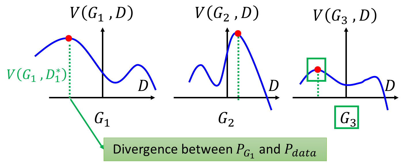
2、max V(G, D)

• Given $G$, what is the optimal $D^{\ast }$ maximizing:
  $$\begin{gathered} V=E_{x{P}_{data}}[logD(x)]+E_{x{P}_G}[log(1-D(x))] \\ ={\int }_x[P_{data}(x)logD(x)+P_G(x)log(1-D(x))]dx \end{gathered}$$
• **Assume that D(x) can be any function, ** given $x$, the optimal $D^{\ast }$ maximizing:
  $$P_{data}(x)logD(x)+P_G(x)log(1-D(x))$$
  令：
  $a=P_{data}(x)b=P_G(x)D=D(x)$
  Find $D^{\ast }$ maximizing: $f(D)=alog(D)+blog(1-D)$

$$\begin{gathered} \frac{df(D)}{dD}=a\times \frac{1}{D}+b\times \frac{1}{1-D}\times (-1)=0 \\ {D}^{\ast }=\frac{a}{a+b} \\ 0<D^{\ast }(x)=\frac{P_{data}(x)}{P_{data}(x)+P_G(x)}<1 \\ {D}^{\ast }(x)=-2log2+2JSD(P_{data}||P_G) \end{gathered}$$

• Jensen-Shannon divergence:
  $$\begin{gathered} JSD(P||Q)=\frac{1}{2}D(P||M)+\frac{1}{2}D(Q||M) \\ M=\frac{1}{2}(P+Q) \end{gathered}$$
  $$\begin{gathered} G^{\ast }=argminmaxV(G,D) \\ {D}^{\ast }=argmaxV(D,G) \end{gathered}$$
  

3、Algorithm

• To find the best $G$ minimizing the loss function $L(G)$:
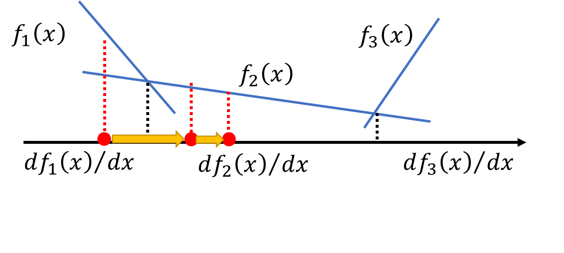
  θ G − η ∂ L ( G ) ∂ θ G → θ G + 1 f ( x ) = m a x { f 1 ( x ) , f 2 ( x ) , f 3 ( x ) } \theta_G - \eta \frac{\partial L(G)}{\partial \theta_G} → \theta_{G + 1}\\ f(x) = max\{f_1(x), f_2(x), f_3(x)\} θG​−η∂θG​∂L(G)​→θG+1​f(x)=max{f1​(x),f2​(x),f3​(x)}
  
• Given $G_0$;
• Find $D_0^{\ast }$ maximizing $V(G_0,D)$(gradient ascent);
• ${\theta }_0-\eta \frac{\partial V(G,D_0^{\ast })}{\partial {\theta }_G}\to G_1$;
• Find $D_1^{\ast }$ maximizing $V(G_1,D)$;

---

二、Framework of GAN

1、f-divergence

$P$ and $Q$ are two distributions. $p(x)$ and $q(x)$ are the probability of sampling $x$. $D_f(P||Q)$ evaluates the difference of $P$ and $Q$.

• $f$ is convex;
• f(1) = 0.
  $$D_f(P||Q)={\int }_{x}q(x)f(\frac{p(x)}{q(x)})dx$$

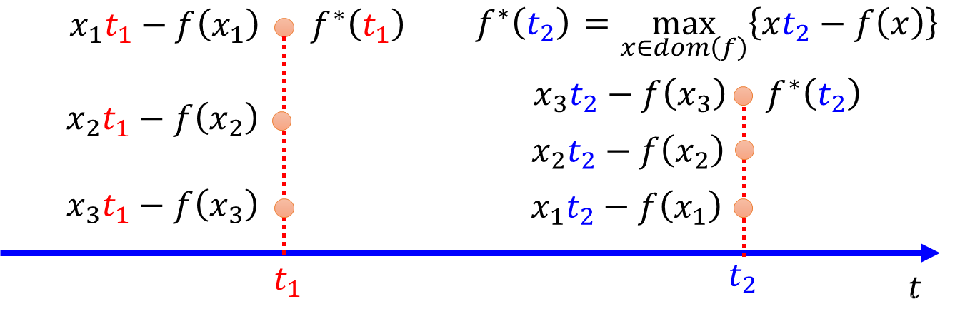
2、Fenchel Conjugate

Every convex function $f$ has a conjugate function (共轭函数) $f^{\ast }$:
f ∗ ( t ) = m a x { x t − f ( x ) } f^*(t) = max\{xt - f(x) \} f∗(t)=max{xt−f(x)}

---

三、Tips for Improving GAN

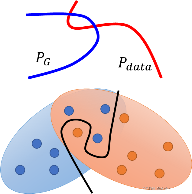
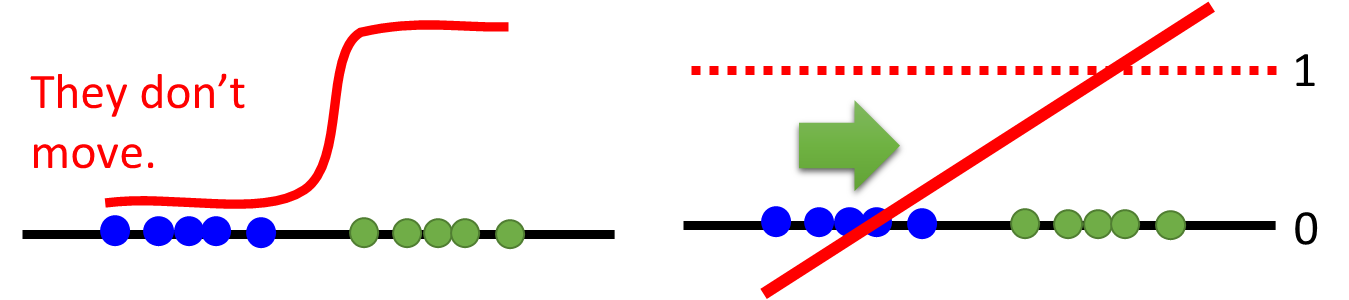
1、JS divergence is not suitable

In most cases, $P_G$ and $P_{data}$ are not overlapped.

2、Least Square GAN（LSGAN）

Replace sigmoid with linear (replace classification with regression).

3、Wasserstein GAN（WGAN）

A “moving plan” is a matrix. Average distance of a plan $\gamma$:
$$B(\gamma )=\sum _{x_p,x_q}\gamma (x_p,x_q)||x_p-x_q||$$
Earth Mover’s Distance:
$$W(P,Q)=minB(\gamma )$$

---