【时间序列预测算法】——Holt-Winters算法介绍及代码实现

背景

一阶二阶三阶指数平滑方法拟合效果均较好，通过结合数据自然属性，数据自身、趋势变化、季节性，提出了这三个角度的衡量量，可以说，理解起来更自然、更亲切。其中三阶的指数平滑方法也被称为“Holt-Winters”算法。

公式

一阶：

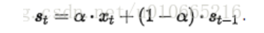
$s_t$是t时刻对$x_t$的估计值，这里只有一个参数α，是数据本身的平滑属性的体现。

二阶：

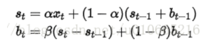
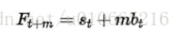
引入了时间趋势变量$b_t$，优化了一下一阶的公式。同时还可以预测t+m时刻的值：

三阶：

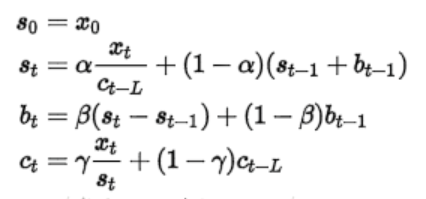
又引入了季节性周期描述变量$c_t$，优化了一下二阶的公式。同时还可以预测t+m时刻的值：

NOTE：$c_{t-L}$我在代码实现时使用的t mod L，因为既然是描述季节性的变量，则其应该体现的是周期L区间内的相对时刻点$t\in [0,L]$，所以应该是取余更合理些，而且代码的执行结果正确，也说明这样实现是可以的。

代码

# 参数设置
s0 = 0
b0 = 0
c0 = 1
# 初始化
# α是数据平滑因子
# β是趋势平滑因子
# γ是季节改变平滑因子
alpha = 0.5
beta = 0.5
gama = 0.5
# 预测长度 预测第t+m时刻
m = 5
# 季节周期长度
L = 5
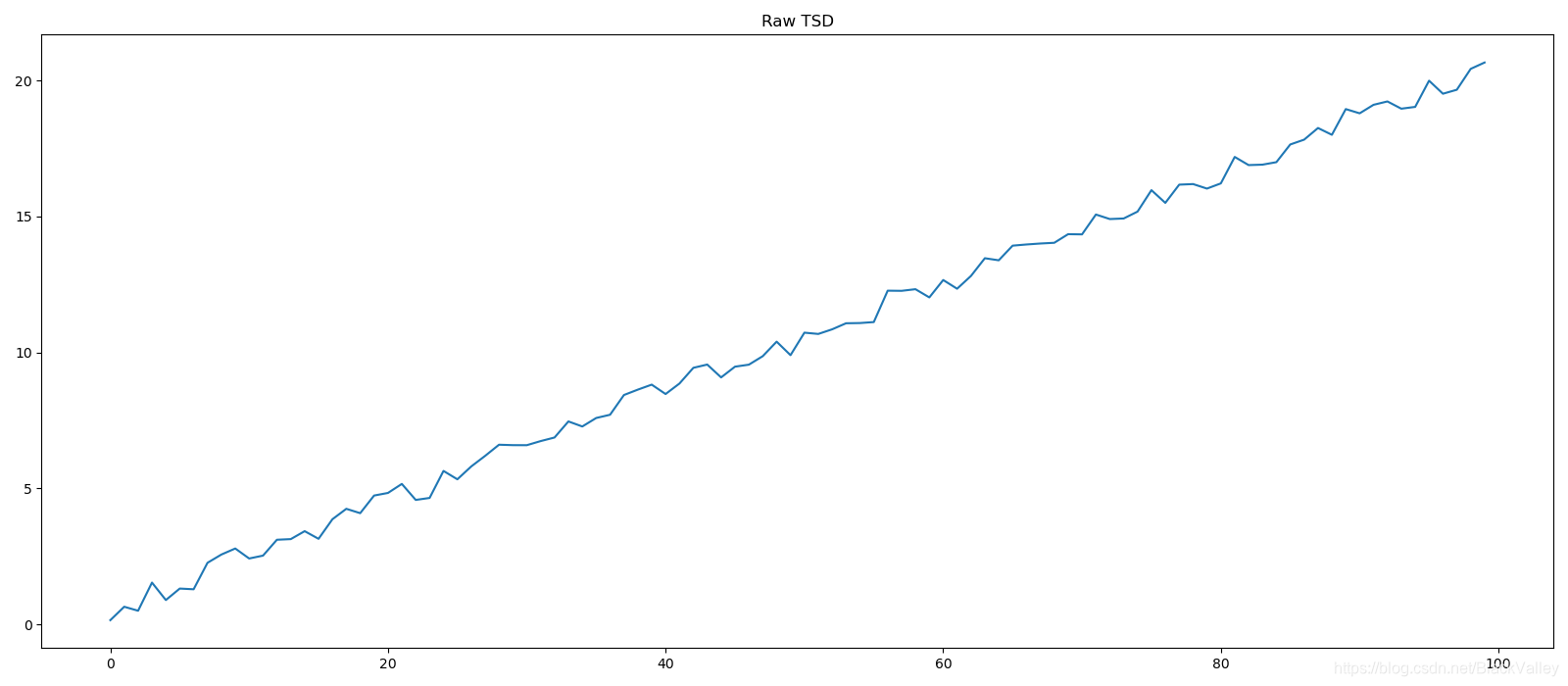
# TSD数据集构造
t = np.linspace(0, 10, 100)
y = 2 * t + np.random.rand(len(t))
# 原始时序数据
plt.figure(figsize=(16, 7))
plt.plot(y)
plt.title("Raw TSD")
plt.show()


# exp smooth order 1
def ExpSmooth(y, s0, alpha, order=1, b0=0, beta=0.5,c0=1,gama=0.5):
    if order == 1:
        s = [s0]
        for i in range(1, len(y)):
            s.append(alpha * y[i] + (1 - alpha) * s[-1])
        return s
    if order == 2:
        s = [s0]
        b = [b0]
        for i in range(1, len(y)):
            s.append(alpha * y[i] + (1 - alpha) * (s[-1] + b[-1]))
            b.append(beta * (s[i] - s[i - 1]) + (1 - beta) * b[-1])
        return s, b
    if order == 3:
        if b0 is None:
            # 初始化趋势估计b0
            sum = 0
            for i in range(L):
                sum+=(y[L+i+1]-y[i+1])
            b0 = sum/(L**2)
        s = [s0]
        b = [b0]
        c = np.ones(L)*c0#c是季节量 固定长度L
        for i in range(1, len(y)):
            c[i % L] = c[i%L] if c[i%L]!=0 else c[i%L]+1e-5
            s.append(alpha * y[i]/(c[i%L]) + (1 - alpha) * (s[-1] + b[-1]))
            b.append(beta * (s[i] - s[i - 1]) + (1 - beta) * b[-1])
            c[i%L] = gama*y[i]/s[i]+(1-gama)*c[i%L]
        return s, b,c
    return None


# for epoch in range(epochs):#暂未找到自动搜索alpha的方法
# print("Epoch:",epoch+1)
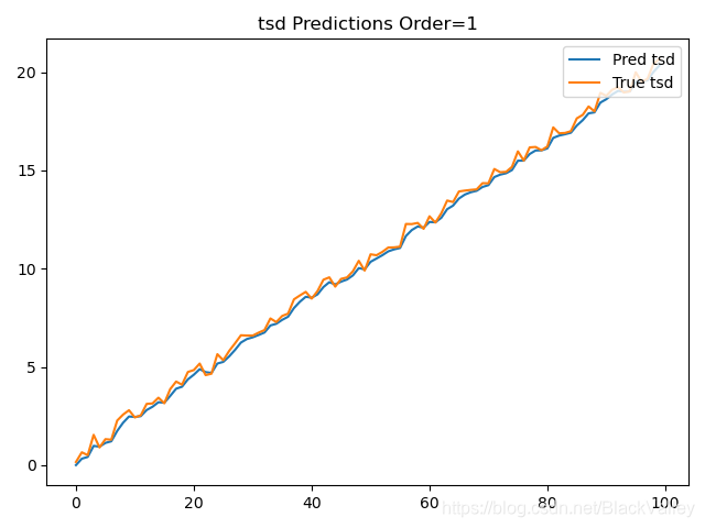
predict = ExpSmooth(y, s0, alpha)
loss = np.mean((predict - y) ** 2)
print("Order=1 loss:", loss, "alpha:", alpha)
plt.plot(predict, label='Pred tsd')
plt.plot(y, label='True tsd')
plt.legend(loc=1)
plt.title("tsd Predictions Order=1")
plt.show()
# b:时间趋势统计量
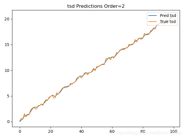
predict, b = ExpSmooth(y, s0, alpha, order=2, b0=b0, beta=beta)
loss = np.mean((predict - y) ** 2)
print("Order=2 loss:", loss, "alpha:", alpha, "beta:", beta)
plt.plot(predict, label='Pred tsd')
plt.plot(y, label='True tsd')
plt.legend(loc=1)
plt.title("tsd Predictions Order=2")
plt.show()
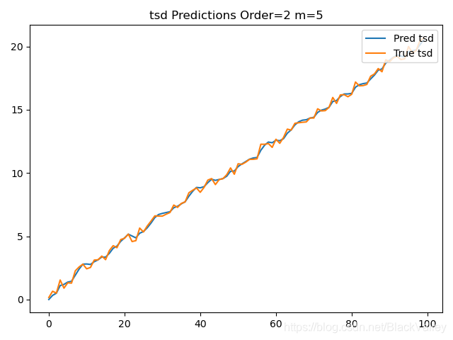
# 二阶指数平滑可以预测t+m时刻的结果
# y[t+m]=predict[t]+mb[t]
predict_m = [predict[t_] + m * b[t_] for t_ in range(len(y) - m)]
loss = np.mean((predict_m - y[m:]) ** 2)
print("Order=2 loss:", loss, "alpha:", alpha, "beta:", beta, "m:", m)
plt.plot(predict, label='Pred tsd')
plt.plot(y, label='True tsd')
plt.legend(loc=1)
plt.title("tsd Predictions Order=2 m=%d" % m)
plt.show()
# Order=3
# 季节性被定义为时间序列数据的周期性。
# “季节”表示行为每隔时间段L就开始重复。
# 季节性“累加性”(additive)和“累乘性“(multiplicative)，就像加法和乘法是数学的基本运算。
# 如果12月都比11月多卖出10套公寓，“累加性”。
# 如果12月都比11月多卖出10%的公寓，“累乘性”。
predict, b,c = ExpSmooth(y, s0, alpha, order=3, b0=b0, beta=beta,c0=c0,gama=gama)
loss = np.mean((predict - y) ** 2)
print("Order=3 loss:", loss, "alpha:", alpha, "beta:", beta)
plt.plot(predict, label='Pred tsd')
plt.plot(y, label='True tsd')
plt.legend(loc=1)
plt.title("tsd Predictions Order=3")
plt.show()
# 三阶指数平滑可以预测t+m时刻的结果
# y[t+m]=(predict[t]+mb[t])c[(t-L+m)%L]
predict_m = [(predict[t_] + m * b[t_])*c[(t_-L+m)%L] for t_ in range(len(y) - m)]
loss = np.mean((predict_m - y[m:]) ** 2)
print("Order=3 loss:", loss, "alpha:", alpha, "beta:", beta, "m:", m)
plt.plot(predict, label='Pred tsd')
plt.plot(y, label='True tsd')
plt.legend(loc=1)
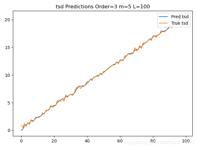
plt.title("tsd Predictions Order=3 m=%d L=%d" % (m,L))
plt.show()

执行结果：

Order=1 loss: 0.07114916427311936 alpha: 0.5
Order=2 loss: 0.04139525147369299 alpha: 0.5 beta: 0.5
Order=2 loss: 0.45574668632556364 alpha: 0.5 beta: 0.5 m: 5
Order=3 loss: 0.8635669515997065 alpha: 0.5 beta: 0.5
Order=3 loss: 0.6321299717453702 alpha: 0.5 beta: 0.5 m: 5

因为原时序数据的季节性体现不出来（一直趋势递增），所以取L=5是不合适的，所以loss较大（三阶时），如果取$L=len(y)$，则

Order=1 loss: 0.07447383143094989 alpha: 0.5
Order=2 loss: 0.042357649823148484 alpha: 0.5 beta: 0.5
Order=2 loss: 0.27533954807136674 alpha: 0.5 beta: 0.5 m: 5
Order=3 loss: 0.042357649823148484 alpha: 0.5 beta: 0.5 gama: 0.5
Order=3 loss: 0.2630090504808384 alpha: 0.5 beta: 0.5 gama: 0.5 m: 5 L: 100

NOTE：因为每次运行时原始tsd都不同（有rand因素），所以loss没有直接的可比性，但可通过观察相对大小关系比较发现，取$L=len(y)$后，loss明显下降，说明可以把无周期性的数据看做周期$T\ge len(y)$的周期性数据。

输出图像：

结论

1. 阶数Order越高，预测loss越小，越准确预测（但不是绝对的）
2. 预测$y_t$后计算$y_{t+m}$的结果（二阶三阶时）比直接预测$y_{t+m}$误差大，但效果也还可以
3. 算法思想核心是引入描述自然属性的变量+递推公式

参考

CSDN博客