分类器的评价指标（ROC、AUC）原理并利用Python+tensorflow举例

最新推荐文章于 2021-04-07 20:20:50 发布

爱吃猫的小鱼干

最新推荐文章于 2021-04-07 20:20:50 发布

阅读量3.4k

点赞数 4

分类专栏： CV Python 文章标签：分类器评价指标 ROC AUC python 机器学习

本文链接：https://blog.csdn.net/BreakingDawn0/article/details/102747447

版权

Python 同时被 2 个专栏收录

8 篇文章 0 订阅

订阅专栏

4 篇文章 1 订阅

订阅专栏

> **获取更多内容，请访问博主的个人博客 [爱吃猫的小鱼干的Blog](https://su-lemon.gitee.io/)**

本文介绍分类器的主要性能指标，介绍ROC和AUC的原理，并以在Tensorflow中利用MNIST数据集训练的手写数字识别模型为例，做出其ROC曲线。

1.基本概念

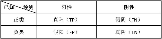
针对一个二分类问题，将实例分成正类(postive)或者负类(negative)。但是实际中分类时，会出现四种情况.，如下表所示：

即：

若一个实例是正类，并且被预测为正类，即为真正（阳）类(True Postive TP)
若一个实例是正类，但是被预测成为负类，即为假负（阴）类(False Negative FN)
若一个实例是负类，但是被预测成为正类，即为假正（阳）类(False Postive FP)
若一个实例是负类，并且被预测成为负类，即为真负（阴）类(True Negative TN)

可以得到分类器的一些性能指标：

精确度 Precision

预测为阳的实例中，原本为正类的比例（越大越好，理想为1）；

P = TP / (TP + FP)

召回率 Recall

原本为正类的实例当中，预测为阳性的比例（越大越好，理想为1）；

R = TP / (TP + FN)

F-measure

F度量是对准确率和召回率做一个权衡（越大越好，理想为1，此时Precision为1，Recall为1）；

F = (2 * Recall * Precision) / (Recall + Precision).

准确率 Accuracy

预测对的（包括原本是正类预测为阳性，原本是负类预测为阴性两种情形）占整个实例的比例（越大越好，理想为1）；

A = (TP + TN) / (TP + TN + FP + FN)

命中率 TPR

TPR = 预测为阳的正类 / 所有正类 = TP / （TP + FN）

假报率 FPR

FPR = 预测为阳的负类 /所有负类 = FP /（FP + TN）

2.ROC曲线

ROC（Receiver Operating Characteristic Curve)，即受试者工作特征曲线。是用来验证一个分类器（二分类）模型的性能的。下图是一个ROC曲线：

要绘制一个ROC曲线，需要命中率(TPR)和假报率(FPR)，ROC曲线中分别将FPR和TPR定义为x和y轴，这样就描述了真阳性(获利)和假阳性(成本)之间的博弈。

（1）ROC曲线中的特殊点和线

(0,1)，即FPR=0, TPR=1，这意味着FN=0，并且FP=0。这是一个完美的分类器，它将所有的样本都正确分类。

(1,0)，即FPR=1，TPR=0，这意味着TP0，并且TN=0。这是一个最糟糕的分类器，因为它成功避开了所有的正确答案。

(0,0)，即FPR=TPR=0，FP=TP=0，该分类器预测所有样本结果都为阴性。

(1,1)，分类器实际上预测所有样本的结果都为阳性。

因此，ROC曲线越接近左上角，该分类器的性能越好。

直线y=x上的点其实表示的是一个采用随机猜测策略分类器的预测结果，例如(0.5,0.5)，表示该分类器随机对于一半的样本预测其为阳性，另，外一半的样本预测为阴性。

（2）如何绘制一个ROC曲线

给定一个初始阈值threshold（一般是从0%开始）
分类器的结果以概率输出（即对一个实例，分类器输出其可能在每类中的概率），pre=[p1,p2,p3...,pn]（n分类）
规定预测概率大于阈值threshold的结果为阳性。对于样本中所有的第一类实例，可以比较p1和threshold计算得到其TPR和FPR，点（FPR，TPR）即为此次threshold下ROC曲线上的一点。同样其它n类实例也可以按该方法得出，这意味着，n分类就会有n条ROC曲线，最后取平均值作为分类器的ROC曲线。
得到一个点后，给一个新的阈值（如每次加1%），并重复步骤2、3，得到下一个点，直到阈值取到100%。
若干个点最后组成了ROC曲线。

（3）AUC

AUC(Area under Curve)：Roc曲线下的面积，介于0和1之间。AUC作为数值可以直观的评价分类器的好坏，值越大越好。

3.ROC曲线绘制举例

使用单个神经元建立模型，通过MNIST手写数据集训练一个可以对手写数字0-9分类的简分类器，绘制它的ROC曲线（是通过逐步计算得到的，实际使用时可以考虑查阅模块中包含的ROC计算函数）。

使用代码时，先注释载入模型之后的内容，使用模型训练部分训练模型；然后注释掉训练部分，使用载入模型部分。

（1）二分类问题的ROC（以对数字0分类为例）

import tensorflow as tf
from tensorflow.examples.tutorials.mnist import input_data
import numpy as np
import pylab
import matplotlib.pyplot as plt
import os

os.environ['TF_CPP_MIN_LOG_LEVEL'] = '2'
mnist = input_data.read_data_sets("MNIST_data/", one_hot=True)

tf.reset_default_graph()

x = tf.placeholder(tf.float32, [None, 784])
y = tf.placeholder(tf.float32, [None, 10])

w = tf.Variable(tf.random_normal(([784, 10])))
b = tf.Variable(tf.zeros(([10])))

pred = tf.nn.softmax(tf.matmul(x, w) + b)  # softmax分类，以概率输出
cost = tf.reduce_mean(
    -tf.reduce_sum(y * tf.log(pred), reduction_indices=1))  # 交叉熵
learning_rate = 0.01
optimizer = tf.train.GradientDescentOptimizer(learning_rate).minimize(cost)

training_epoch = 25
batch_size = 100  # 每一批次的训练数据量
display_step = 1

saver = tf.train.Saver()
model_path = "log/digital_recognition/digital_recognition.ckpt"

"""# 训练模型
with tf.Session() as sess:
    sess.run(tf.global_variables_initializer())

    # 启动循环开始训练
    for epoch in range(training_epoch):
        avg_cost = 0
        total_batch = int(mnist.train.num_examples / batch_size)

        # 训练所有的数据集
        for batch in range(total_batch):
            batch_xs, batch_ys = mnist.train.next_batch(batch_size)

            _, c = sess.run([optimizer, cost],
                            feed_dict={x: batch_xs, y: batch_ys})
            avg_cost += c / total_batch  # 平均损失值

        # 按display_step显示训练得信息
        if (epoch + 1) % display_step == 0:
            print("Epoch:", '%04d' % (epoch + 1), "cost=",
                  "{:.9E}".format(avg_cost))
    print("Train Finished!")

    # 测试模型
    corr_pre = tf.equal(tf.argmax(pred, 1), tf.argmax(y, 1))
    accuracy = tf.reduce_mean(tf.cast(corr_pre, tf.float32))
    print("Accuracy:",
          accuracy.eval({x: mnist.test.images, y: mnist.test.labels}))

    # 保存模型
    save_path = saver.save(sess, model_path)
    print("Model saved in file: %s" % save_path)"""

threshold = 0  # 阈值
threshold_step = 0.05  # 阈值增量
test_size = 2000
TPRs, FPRs = [], []

# 载入模型
print("\nStart 2nd session")
with tf.Session() as sess:
    sess.run(tf.global_variables_initializer())  # 初始化变量
    saver.restore(sess, model_path)  # 恢复模型变量

    # 预测
    output = tf.argmax(pred, 1)
    batch_xs, batch_ys = mnist.train.next_batch(test_size)  # 从数据集返回实例
    output_val, pre_val = sess.run([output, pred], feed_dict={x: batch_xs})
    print(output_val, "\n", pre_val, "\n", pre_val[1, 0], "\n", batch_ys)

    # 逐次计算TPR，FPR
    while threshold <= 1.0:
        TP, FN, FP, TN = 0, 0, 0, 0
        # 计算分类器预测数字0时的TP，FP，TN，FN
        for i in range(test_size):
            if pre_val[i, 0] > threshold and int(batch_ys[i, 0]) == 1:
                TP += 1
            elif pre_val[i, 0] > threshold and int(batch_ys[i, 0]) == 0:
                FP += 1
            elif pre_val[i, 0] <= threshold and int(batch_ys[i, 0]) == 1:
                FN += 1
            elif pre_val[i, 0] <= threshold and int(batch_ys[i, 0]) == 0:
                TN += 1
        TPRs.append(TP / (TP + FN))
        FPRs.append(FP / (FP + TN))
        threshold += threshold_step

    plt.step(FPRs, TPRs, label="num 0 ROC")
    plt.plot(np.linspace(0, 1, 20), np.linspace(0, 1, 20))
    plt.xlabel("FPR")
    plt.ylabel("TPR")
    plt.xlim(0, 1)
    plt.ylim(0, 1)
    plt.legend()
    plt.show()
    plt.savefig("D:\\_Picture Files\\其他\\1.png")

（2）多分类问题的ROC（数字0-9分类）

同样，如果没有模型，需要先用上文代码训练模型。

threshold = 0  # 阈值
threshold_step = 0.05  # 阈值增量
test_size = 2000

# 载入模型
print("\nStart 2nd session")
with tf.Session() as sess:
    sess.run(tf.global_variables_initializer())  # 初始化变量
    saver.restore(sess, model_path)  # 恢复模型变量

    # 预测
    output = tf.argmax(pred, 1)
    batch_xs, batch_ys = mnist.train.next_batch(test_size)  # 从数据集返回下2个实例
    output_val, pre_val = sess.run([output, pred], feed_dict={x: batch_xs})
    print(output_val, "\n", pre_val, "\n", pre_val[1, 0], "\n", batch_ys)

    # 对每个数的预测计算TPR，FPR
    for num in range(10):
        TPRs, FPRs = [], []
        threshold = 0
        # 逐次计算TPR，FPR
        while threshold <= 1.0:
            TP, FN, FP, TN = 0, 0, 0, 0
            for i in range(test_size):
                if pre_val[i, num] > threshold and int(batch_ys[i, num]) == 1:
                    TP += 1
                elif pre_val[i, num] > threshold and int(batch_ys[i, num]) == 0:
                    FP += 1
                elif pre_val[i, num] <= threshold and int(batch_ys[i, num]) == 1:
                    FN += 1
                elif pre_val[i, num] <= threshold and int(batch_ys[i, num]) == 0:
                    TN += 1
            TPRs.append(TP / (TP + FN))
            FPRs.append(FP / (FP + TN))
            threshold += threshold_step

        label_str = "num" + str(num) + "ROC"
        plt.step(FPRs, TPRs, label=label_str)

    plt.plot(np.linspace(0, 1, 20), np.linspace(0, 1, 20))
    plt.xlabel("FPR")
    plt.ylabel("TPR")
    plt.xlim(0, 1)
    plt.ylim(0, 1)
    plt.legend()
    plt.savefig("D:\\_Picture Files\\其他\\1.png")
    plt.show()

分类器的ROC对10条曲线取平均即可

（3）AUC的意义

一个合适的分类器，要求做到TPR较高而FPR较小，在ROC曲线上，就是在相同的FPR时，TPR越大的越好。

在比较分类器的性能时，如果一条ROC始终在另一条ROC曲线之上（图中num1，num8），很好判断分类的好坏；但某些情况下，两条曲线相交，这就很难进行判断到底哪个分类器性能好。

所以我们用AUC进行评价。AUC的值等于ROC曲线与FPR轴线形成的面积。AUC的值越大越好，其取值:

=1，完美的分类，不存在；
（0.5,1），分类效果优于随机分类；
<0.5分类效果比不上随机分类。

> **获取更多内容，请访问博主的个人博客 [爱吃猫的小鱼干的Blog](https://su-lemon.gitee.io/)**

爱吃猫的小鱼干

关注

4
点赞
踩
35

收藏

觉得还不错? 一键收藏
1
评论
分类器的评价指标（ROC、AUC）原理并利用Python+tensorflow举例

本文介绍分类器的主要性能指标，介绍ROC和AUC的原理，并以在Tensorflow中利用MNIST数据集训练的手写数字识别模型为例，做出其ROC曲线。1.基本概念针对一个二分类问题，将实例分成正类(postive)或者负类(negative)。但是实际中分类时，会出现四种情况.，如下表所示：即：若一个实例是正类，并且被预测为正类，即为真正（阳）类(True Postive TP...
复制链接

扫一扫