MobileNetV2：Inverted Residuals and Linear Bottlenecks

MobileNetV2: Inverted Residuals and Linear Bottlenecks

MobileNetV2：反向残差(逆向残差)和线性瓶颈

发表时间：[Submitted on 13 Jan 2018 (v1, last revised 21 Mar 2019 (this version, v4)]

发表期刊/会议：Computer Vision and Pattern Recognition

论文地址：https://arxiv.org/abs/1801.04381；

代码地址：；

关键词：MobileNetV1延伸 逆向残差 线性瓶颈

---

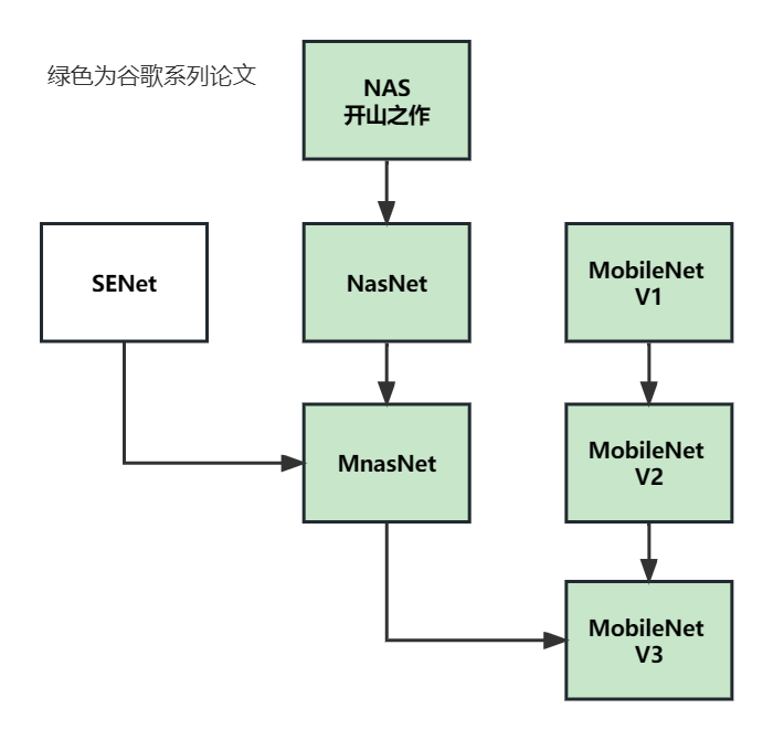
系列论文阅读顺序：

---

0 摘要

①本文提出了一种新的移动端架构MobileNet V2，在当前移动端模型中最优；

②本文介绍了一种新框架：SSDLite，描述了如何通过SSDLite将这些移动模型应用于对象检测；（不重要）

③本文还演示了如何通过简化形式的DeepLabv3（称之为mobile DeepLabv3）构建移动端的语义分割模型；（不重要）

MobileNetV2 架构基于反向残差结构(inverted residual structure)全文重点；

最后在分类/目标检测/图像分割任务中评估了MobileNetV2的性能；

1 简介

CNN提高准确性的代价往往是消耗大量的计算资源。

本文介绍了一种新的神经网络架构，该架构专门针对移动端和资源受限的环境（比如手机、监控摄像头等），该网络通过显著减少所需的操作和内存数量，同时保持相同的准确性，推动了移动端定制计算机视觉模型的最新技术。

本文主要贡献是一个新的层模块：具有线性瓶颈的逆向残差。该模块输入为低维特征，首先将其扩展到高维，并使用轻量级深度卷积进行滤波。

(说人话：一般方法是先降维后升维，本文先升维，后降维。为什么呢？section 3中具体解释为什么)；

2 相关工作

CNN在准确性与性能之间平衡的相关工作；

3 Preliminaries, discussion and intuition

3.1 深度可分离卷积

详情见MobileNet V1；

图2：(左)标准卷积核的分解；(右)示例；

3.2 线性瓶颈

对于输入CNN的数据，我们把CNN中所有激活层形成的输出叫做"感兴趣的流形"(manifold of interest)；人们一直认为神经网络中"感兴趣的流形"可以嵌入到低维子空间中。

这一信息可以通过降维来捕获和利用，比如MobileNet V1中，已经成功利用这一点，通过宽度乘数参数α在计算精度和效率之间取得平衡。

(说人话：特征降维之后主要信息仍然会保留，降维去除冗余信息对正确率影响不大，并且可以减少参数量，提高效率。)

BUT…

当我们想起CNN实际上具有非线性变换（如ReLU）时，这种直觉就崩溃了。比如，当ReLU应用于一维空间时会产生“射线”，应用于n维空间时，会产生具有n个节点的曲线；如图1具体展示：

图1：嵌入高维空间中的低维流形的ReLU变换示例。

输入一个螺旋形的张量(典型二维空间，实际就是一堆(x,y)坐标，非线性问题)，经过矩阵T变换和ReLU激活后，降维到不同的维度输出并可视化，从图1中可以看出：

• 维度越低，比如 n = 2,3时，损失信息非常多(2和3已经没有螺旋的样子了)；

• 维度越高，损失信息越少，n = 15,30最接近输入；

说人话：

• 过渡降维会导致信息丢失，接着用ReLU函数也会导致小于0的部分信息丢失，但是强大的CNN又离不开非线性激活函数(比如ReLU)，线性激活CNN只能识别一维空间；
• 所以要先保留冗余的维度进行ReLU，防止信息丢失，也同时能发挥ReLU非线性激活函数的作用；
• 所以要先升维，再降维。（回答section1提出的问题 为了避免信息丢失）

文章强调了两个见解：

• 1：如果"感兴趣的流形"在ReLU变换后保持非零体积，则它对应于线性变换（说人话：如果"manifold of interest"都为正，则经过ReLU相当于做了一个线性变换，没有信息丢失）；
• 2：ReLU能够保存关于"感兴趣的流形"的完整信息，仅当输入流形位于输入空间的低维子空间中时（当维度足够多时，ReLU能够保留"manifold of interest"的完整信息）；

以上两个见解为我们提供了优化现有神经架构的经验提示：假设"感兴趣的流形"是低维的，我们可以通过在卷积块中插入线性瓶颈层(linear bottleneck)来捕捉这一点。实验证据表明，使用线性层至关重要，因为它可以防止非线性破坏太多信息。

为了减少信息丢失，本文提出了linear bottleneck，就是在bottlenck(1 × 1卷积)的最后输出不接非线性激活层，只做linear操作；

图2：可分离卷积块的演化。

2(a)：标准卷积（一个大方块）；

2(b)：深度可分离卷积(=Depthwise convolution+Pointwise Convolution=薄片片+方块块)；

2(c )：【linear bottleneck】(高维后)relu6-dw-relu6-pw降维-升维-；

2(d)：和图2(c )等效，(线性激活后)pw升维-relu6-dw-relu6-pw降维-线性激活；

3.3 反向残差(逆向残差)

3.3.1 图解

图3显示了残差连接和反向残差连接的差异。

反向残差的设计大大提高了内存效率，并且在本文的实验中效果稍好。

图3：残差块和逆向残差之间的差异。图3(a)：pw降维-3*3卷积-pw升维(经典的先降维后升维)；图3(b)：pw升维-dw-pw降维-线性激活(逆向残差，先升维后降维)；注意图方块的大小和残差连接的位置，大方块代表高维度，小方块代表低维度；一般残差块连接两个高维度，逆向残差块连接两个低维度； 表1：逆向残差实现架构

表1解释：
扩展因子：$t$；

stride：$s$；

①输入：$h\times w\times k$----pw升维到$h\times w\times tk$；
②经过dw，维度不变h,w根据s变化为$\frac{h}{s}\times \frac{w}{s}\times (tk)$；
③线性激活到$\frac{h}{s}\times \frac{w}{s}\times k^{\prime }$；

3.3.2 反向残差代码

class InvertedResidual(nn.Module):
    def __init__(self, in_channel, out_channel, stride, expand_ratio):
        super(InvertedResidual, self).__init__()
        # expand_ratio: 扩展因子t
        # in_channel:k
        # 输出通道数: tk
        hidden_channel = in_channel * expand_ratio
        self.use_shortcut = stride == 1 and in_channel == out_channel

        # 将所有层保存为一个list
        layers = []
        if expand_ratio != 1:
            # 1x1 pw 接ReLU激活(非线性)
            layers.append(ConvBNReLU(in_channel, hidden_channel, kernel_size=1))
        layers.extend([
            # 3x3 dw
            ConvBNReLU(hidden_channel, hidden_channel, stride=stride, groups=hidden_channel),
            # 1x1 pw 与一个层不同 这层后接线性激活
            nn.Conv2d(hidden_channel, out_channel, kernel_size=1, bias=False),
            nn.BatchNorm2d(out_channel),
        ])

        self.conv = nn.Sequential(*layers)

    def forward(self, x):
        if self.use_shortcut:
            return x + self.conv(x)
        else:
            return self.conv(x)

class ConvBNReLU(nn.Sequential):
    def __init__(self, in_channel, out_channel, kernel_size=3, stride=1, groups=1):#groups=1普通卷积
        padding = (kernel_size - 1) // 2
        super(ConvBNReLU, self).__init__(
            nn.Conv2d(in_channel, out_channel, kernel_size, stride, padding, groups=groups, bias=False),
            nn.BatchNorm2d(out_channel),
            nn.ReLU6(inplace=True)
        )

4 模型架构

4.1 模型架构概述

表2描述了MobileNet V2的完整架构；

表2：MobileNet V2实现架构。t：扩展因子；c：通道数；n：该层重复次数；s：步幅；卷积核大小均为3 * 3;

本文使用ReLU6作为非线性激活函数，训练过程使用dropout和batch normalization；

除了第一层，在整个网络中使用恒定的扩展因子t；较小的网络用较小的扩展因子t表现更好；较大的网络使用较大的扩展因子时表现更好。

MobileNet v2同样使用MobileNet V1中的两个超参数，宽度系数α和分辨率系数ρ；

4.2 架构代码

class MobileNetV2(nn.Module):
    def __init__(self, num_classes=1000, alpha=1.0, round_nearest=8):#alpha超参数
        super(MobileNetV2, self).__init__()
        block = InvertedResidual
        # _make_divisible 函数确保为 8 的整数倍
        # 为什么?
        # 为了快，8，16，24...这些 size 符合处理器单元的对齐位宽(硬件角度)
        input_channel = _make_divisible(32 * alpha, round_nearest)
        last_channel = _make_divisible(1280 * alpha, round_nearest)

        # 定义7个bottleneck的一些参数
        # 对照原文表2
        inverted_residual_setting = [
            # t, c, n, s
            [1, 16, 1, 1],
            [6, 24, 2, 2],
            [6, 32, 3, 2],
            [6, 64, 4, 2],
            [6, 96, 3, 1],
            [6, 160, 3, 2],
            [6, 320, 1, 1],
        ]

        # 保存层
        features = []
        # conv1 layer
        features.append(ConvBNReLU(3, input_channel, stride=2))

        # 逆向残差块
        for t, c, n, s in inverted_residual_setting:
            output_channel = _make_divisible(c * alpha, round_nearest)
            for i in range(n):
                stride = s if i == 0 else 1
                features.append(block(input_channel, output_channel, stride, expand_ratio=t))
                input_channel = output_channel
        # building last several layers
        features.append(ConvBNReLU(input_channel, last_channel, 1))
        # combine feature layers
        self.features = nn.Sequential(*features)

        # building classifier
        self.avgpool = nn.AdaptiveAvgPool2d((1, 1))
        self.classifier = nn.Sequential(
            nn.Dropout(0.2),
            nn.Linear(last_channel, num_classes)
        )

        # weight initialization
        for m in self.modules():
            if isinstance(m, nn.Conv2d):
                nn.init.kaiming_normal_(m.weight, mode='fan_out')
                if m.bias is not None:
                    nn.init.zeros_(m.bias)
            elif isinstance(m, nn.BatchNorm2d):
                nn.init.ones_(m.weight)
                nn.init.zeros_(m.bias)
            elif isinstance(m, nn.Linear):
                nn.init.normal_(m.weight, 0, 0.01)
                nn.init.zeros_(m.bias)

    def forward(self, x):
        x = self.features(x)
        x = self.avgpool(x)
        x = torch.flatten(x, 1)
        x = self.classifier(x)
        return x

MobileNetV2(
  (features): Sequential(
    (0): ConvBNReLU(
      (0): Conv2d(3, 32, kernel_size=(3, 3), stride=(2, 2), padding=(1, 1), bias=False)
      (1): BatchNorm2d(32, eps=1e-05, momentum=0.1, affine=True, track_running_stats=True)
      (2): ReLU6(inplace=True)
    )
    (1): InvertedResidual(
      (conv): Sequential(
        (0): ConvBNReLU(
          (0): Conv2d(32, 32, kernel_size=(3, 3), stride=(1, 1), padding=(1, 1), groups=32, bias=False)
          (1): BatchNorm2d(32, eps=1e-05, momentum=0.1, affine=True, track_running_stats=True)
          (2): ReLU6(inplace=True)
        )
        (1): Conv2d(32, 16, kernel_size=(1, 1), stride=(1, 1), bias=False)
        (2): BatchNorm2d(16, eps=1e-05, momentum=0.1, affine=True, track_running_stats=True)
      )
    )
    (2): InvertedResidual(
      (conv): Sequential(
        (0): ConvBNReLU(
          (0): Conv2d(16, 96, kernel_size=(1, 1), stride=(1, 1), bias=False)
          (1): BatchNorm2d(96, eps=1e-05, momentum=0.1, affine=True, track_running_stats=True)
          (2): ReLU6(inplace=True)
        )
        (1): ConvBNReLU(
          (0): Conv2d(96, 96, kernel_size=(3, 3), stride=(2, 2), padding=(1, 1), groups=96, bias=False)
          (1): BatchNorm2d(96, eps=1e-05, momentum=0.1, affine=True, track_running_stats=True)
          (2): ReLU6(inplace=True)
        )
        (2): Conv2d(96, 24, kernel_size=(1, 1), stride=(1, 1), bias=False)
        (3): BatchNorm2d(24, eps=1e-05, momentum=0.1, affine=True, track_running_stats=True)
      )
    )
    (3): InvertedResidual(
      (conv): Sequential(
        (0): ConvBNReLU(
          (0): Conv2d(24, 144, kernel_size=(1, 1), stride=(1, 1), bias=False)
          (1): BatchNorm2d(144, eps=1e-05, momentum=0.1, affine=True, track_running_stats=True)
          (2): ReLU6(inplace=True)
        )
        (1): ConvBNReLU(
          (0): Conv2d(144, 144, kernel_size=(3, 3), stride=(1, 1), padding=(1, 1), groups=144, bias=False)
          (1): BatchNorm2d(144, eps=1e-05, momentum=0.1, affine=True, track_running_stats=True)
          (2): ReLU6(inplace=True)
        )
        (2): Conv2d(144, 24, kernel_size=(1, 1), stride=(1, 1), bias=False)
        (3): BatchNorm2d(24, eps=1e-05, momentum=0.1, affine=True, track_running_stats=True)
      )
    )
    (4): InvertedResidual(
      (conv): Sequential(
        (0): ConvBNReLU(
          (0): Conv2d(24, 144, kernel_size=(1, 1), stride=(1, 1), bias=False)
          (1): BatchNorm2d(144, eps=1e-05, momentum=0.1, affine=True, track_running_stats=True)
          (2): ReLU6(inplace=True)
        )
        (1): ConvBNReLU(
          (0): Conv2d(144, 144, kernel_size=(3, 3), stride=(2, 2), padding=(1, 1), groups=144, bias=False)
          (1): BatchNorm2d(144, eps=1e-05, momentum=0.1, affine=True, track_running_stats=True)
          (2): ReLU6(inplace=True)
        )
        (2): Conv2d(144, 32, kernel_size=(1, 1), stride=(1, 1), bias=False)
        (3): BatchNorm2d(32, eps=1e-05, momentum=0.1, affine=True, track_running_stats=True)
      )
    )
    (5): InvertedResidual(
      (conv): Sequential(
        (0): ConvBNReLU(
          (0): Conv2d(32, 192, kernel_size=(1, 1), stride=(1, 1), bias=False)
          (1): BatchNorm2d(192, eps=1e-05, momentum=0.1, affine=True, track_running_stats=True)
          (2): ReLU6(inplace=True)
        )
        (1): ConvBNReLU(
          (0): Conv2d(192, 192, kernel_size=(3, 3), stride=(1, 1), padding=(1, 1), groups=192, bias=False)
          (1): BatchNorm2d(192, eps=1e-05, momentum=0.1, affine=True, track_running_stats=True)
          (2): ReLU6(inplace=True)
        )
        (2): Conv2d(192, 32, kernel_size=(1, 1), stride=(1, 1), bias=False)
        (3): BatchNorm2d(32, eps=1e-05, momentum=0.1, affine=True, track_running_stats=True)
      )
    )
    (6): InvertedResidual(
      (conv): Sequential(
        (0): ConvBNReLU(
          (0): Conv2d(32, 192, kernel_size=(1, 1), stride=(1, 1), bias=False)
          (1): BatchNorm2d(192, eps=1e-05, momentum=0.1, affine=True, track_running_stats=True)
          (2): ReLU6(inplace=True)
        )
        (1): ConvBNReLU(
          (0): Conv2d(192, 192, kernel_size=(3, 3), stride=(1, 1), padding=(1, 1), groups=192, bias=False)
          (1): BatchNorm2d(192, eps=1e-05, momentum=0.1, affine=True, track_running_stats=True)
          (2): ReLU6(inplace=True)
        )
        (2): Conv2d(192, 32, kernel_size=(1, 1), stride=(1, 1), bias=False)
        (3): BatchNorm2d(32, eps=1e-05, momentum=0.1, affine=True, track_running_stats=True)
      )
    )
    (7): InvertedResidual(
      (conv): Sequential(
        (0): ConvBNReLU(
          (0): Conv2d(32, 192, kernel_size=(1, 1), stride=(1, 1), bias=False)
          (1): BatchNorm2d(192, eps=1e-05, momentum=0.1, affine=True, track_running_stats=True)
          (2): ReLU6(inplace=True)
        )
        (1): ConvBNReLU(
          (0): Conv2d(192, 192, kernel_size=(3, 3), stride=(2, 2), padding=(1, 1), groups=192, bias=False)
          (1): BatchNorm2d(192, eps=1e-05, momentum=0.1, affine=True, track_running_stats=True)
          (2): ReLU6(inplace=True)
        )
        (2): Conv2d(192, 64, kernel_size=(1, 1), stride=(1, 1), bias=False)
        (3): BatchNorm2d(64, eps=1e-05, momentum=0.1, affine=True, track_running_stats=True)
      )
    )
    (8): InvertedResidual(
      (conv): Sequential(
        (0): ConvBNReLU(
          (0): Conv2d(64, 384, kernel_size=(1, 1), stride=(1, 1), bias=False)
          (1): BatchNorm2d(384, eps=1e-05, momentum=0.1, affine=True, track_running_stats=True)
          (2): ReLU6(inplace=True)
        )
        (1): ConvBNReLU(
          (0): Conv2d(384, 384, kernel_size=(3, 3), stride=(1, 1), padding=(1, 1), groups=384, bias=False)
          (1): BatchNorm2d(384, eps=1e-05, momentum=0.1, affine=True, track_running_stats=True)
          (2): ReLU6(inplace=True)
        )
        (2): Conv2d(384, 64, kernel_size=(1, 1), stride=(1, 1), bias=False)
        (3): BatchNorm2d(64, eps=1e-05, momentum=0.1, affine=True, track_running_stats=True)
      )
    )
    (9): InvertedResidual(
      (conv): Sequential(
        (0): ConvBNReLU(
          (0): Conv2d(64, 384, kernel_size=(1, 1), stride=(1, 1), bias=False)
          (1): BatchNorm2d(384, eps=1e-05, momentum=0.1, affine=True, track_running_stats=True)
          (2): ReLU6(inplace=True)
        )
        (1): ConvBNReLU(
          (0): Conv2d(384, 384, kernel_size=(3, 3), stride=(1, 1), padding=(1, 1), groups=384, bias=False)
          (1): BatchNorm2d(384, eps=1e-05, momentum=0.1, affine=True, track_running_stats=True)
          (2): ReLU6(inplace=True)
        )
        (2): Conv2d(384, 64, kernel_size=(1, 1), stride=(1, 1), bias=False)
        (3): BatchNorm2d(64, eps=1e-05, momentum=0.1, affine=True, track_running_stats=True)
      )
    )
    (10): InvertedResidual(
      (conv): Sequential(
        (0): ConvBNReLU(
          (0): Conv2d(64, 384, kernel_size=(1, 1), stride=(1, 1), bias=False)
          (1): BatchNorm2d(384, eps=1e-05, momentum=0.1, affine=True, track_running_stats=True)
          (2): ReLU6(inplace=True)
        )
        (1): ConvBNReLU(
          (0): Conv2d(384, 384, kernel_size=(3, 3), stride=(1, 1), padding=(1, 1), groups=384, bias=False)
          (1): BatchNorm2d(384, eps=1e-05, momentum=0.1, affine=True, track_running_stats=True)
          (2): ReLU6(inplace=True)
        )
        (2): Conv2d(384, 64, kernel_size=(1, 1), stride=(1, 1), bias=False)
        (3): BatchNorm2d(64, eps=1e-05, momentum=0.1, affine=True, track_running_stats=True)
      )
    )
    (11): InvertedResidual(
      (conv): Sequential(
        (0): ConvBNReLU(
          (0): Conv2d(64, 384, kernel_size=(1, 1), stride=(1, 1), bias=False)
          (1): BatchNorm2d(384, eps=1e-05, momentum=0.1, affine=True, track_running_stats=True)
          (2): ReLU6(inplace=True)
        )
        (1): ConvBNReLU(
          (0): Conv2d(384, 384, kernel_size=(3, 3), stride=(1, 1), padding=(1, 1), groups=384, bias=False)
          (1): BatchNorm2d(384, eps=1e-05, momentum=0.1, affine=True, track_running_stats=True)
          (2): ReLU6(inplace=True)
        )
        (2): Conv2d(384, 96, kernel_size=(1, 1), stride=(1, 1), bias=False)
        (3): BatchNorm2d(96, eps=1e-05, momentum=0.1, affine=True, track_running_stats=True)
      )
    )
    (12): InvertedResidual(
      (conv): Sequential(
        (0): ConvBNReLU(
          (0): Conv2d(96, 576, kernel_size=(1, 1), stride=(1, 1), bias=False)
          (1): BatchNorm2d(576, eps=1e-05, momentum=0.1, affine=True, track_running_stats=True)
          (2): ReLU6(inplace=True)
        )
        (1): ConvBNReLU(
          (0): Conv2d(576, 576, kernel_size=(3, 3), stride=(1, 1), padding=(1, 1), groups=576, bias=False)
          (1): BatchNorm2d(576, eps=1e-05, momentum=0.1, affine=True, track_running_stats=True)
          (2): ReLU6(inplace=True)
        )
        (2): Conv2d(576, 96, kernel_size=(1, 1), stride=(1, 1), bias=False)
        (3): BatchNorm2d(96, eps=1e-05, momentum=0.1, affine=True, track_running_stats=True)
      )
    )
    (13): InvertedResidual(
      (conv): Sequential(
        (0): ConvBNReLU(
          (0): Conv2d(96, 576, kernel_size=(1, 1), stride=(1, 1), bias=False)
          (1): BatchNorm2d(576, eps=1e-05, momentum=0.1, affine=True, track_running_stats=True)
          (2): ReLU6(inplace=True)
        )
        (1): ConvBNReLU(
          (0): Conv2d(576, 576, kernel_size=(3, 3), stride=(1, 1), padding=(1, 1), groups=576, bias=False)
          (1): BatchNorm2d(576, eps=1e-05, momentum=0.1, affine=True, track_running_stats=True)
          (2): ReLU6(inplace=True)
        )
        (2): Conv2d(576, 96, kernel_size=(1, 1), stride=(1, 1), bias=False)
        (3): BatchNorm2d(96, eps=1e-05, momentum=0.1, affine=True, track_running_stats=True)
      )
    )
    (14): InvertedResidual(
      (conv): Sequential(
        (0): ConvBNReLU(
          (0): Conv2d(96, 576, kernel_size=(1, 1), stride=(1, 1), bias=False)
          (1): BatchNorm2d(576, eps=1e-05, momentum=0.1, affine=True, track_running_stats=True)
          (2): ReLU6(inplace=True)
        )
        (1): ConvBNReLU(
          (0): Conv2d(576, 576, kernel_size=(3, 3), stride=(2, 2), padding=(1, 1), groups=576, bias=False)
          (1): BatchNorm2d(576, eps=1e-05, momentum=0.1, affine=True, track_running_stats=True)
          (2): ReLU6(inplace=True)
        )
        (2): Conv2d(576, 160, kernel_size=(1, 1), stride=(1, 1), bias=False)
        (3): BatchNorm2d(160, eps=1e-05, momentum=0.1, affine=True, track_running_stats=True)
      )
    )
    (15): InvertedResidual(
      (conv): Sequential(
        (0): ConvBNReLU(
          (0): Conv2d(160, 960, kernel_size=(1, 1), stride=(1, 1), bias=False)
          (1): BatchNorm2d(960, eps=1e-05, momentum=0.1, affine=True, track_running_stats=True)
          (2): ReLU6(inplace=True)
        )
        (1): ConvBNReLU(
          (0): Conv2d(960, 960, kernel_size=(3, 3), stride=(1, 1), padding=(1, 1), groups=960, bias=False)
          (1): BatchNorm2d(960, eps=1e-05, momentum=0.1, affine=True, track_running_stats=True)
          (2): ReLU6(inplace=True)
        )
        (2): Conv2d(960, 160, kernel_size=(1, 1), stride=(1, 1), bias=False)
        (3): BatchNorm2d(160, eps=1e-05, momentum=0.1, affine=True, track_running_stats=True)
      )
    )
    (16): InvertedResidual(
      (conv): Sequential(
        (0): ConvBNReLU(
          (0): Conv2d(160, 960, kernel_size=(1, 1), stride=(1, 1), bias=False)
          (1): BatchNorm2d(960, eps=1e-05, momentum=0.1, affine=True, track_running_stats=True)
          (2): ReLU6(inplace=True)
        )
        (1): ConvBNReLU(
          (0): Conv2d(960, 960, kernel_size=(3, 3), stride=(1, 1), padding=(1, 1), groups=960, bias=False)
          (1): BatchNorm2d(960, eps=1e-05, momentum=0.1, affine=True, track_running_stats=True)
          (2): ReLU6(inplace=True)
        )
        (2): Conv2d(960, 160, kernel_size=(1, 1), stride=(1, 1), bias=False)
        (3): BatchNorm2d(160, eps=1e-05, momentum=0.1, affine=True, track_running_stats=True)
      )
    )
    (17): InvertedResidual(
      (conv): Sequential(
        (0): ConvBNReLU(
          (0): Conv2d(160, 960, kernel_size=(1, 1), stride=(1, 1), bias=False)
          (1): BatchNorm2d(960, eps=1e-05, momentum=0.1, affine=True, track_running_stats=True)
          (2): ReLU6(inplace=True)
        )
        (1): ConvBNReLU(
          (0): Conv2d(960, 960, kernel_size=(3, 3), stride=(1, 1), padding=(1, 1), groups=960, bias=False)
          (1): BatchNorm2d(960, eps=1e-05, momentum=0.1, affine=True, track_running_stats=True)
          (2): ReLU6(inplace=True)
        )
        (2): Conv2d(960, 320, kernel_size=(1, 1), stride=(1, 1), bias=False)
        (3): BatchNorm2d(320, eps=1e-05, momentum=0.1, affine=True, track_running_stats=True)
      )
    )
    (18): ConvBNReLU(
      (0): Conv2d(320, 1280, kernel_size=(1, 1), stride=(1, 1), bias=False)
      (1): BatchNorm2d(1280, eps=1e-05, momentum=0.1, affine=True, track_running_stats=True)
      (2): ReLU6(inplace=True)
    )
  )
  (avgpool): AdaptiveAvgPool2d(output_size=(1, 1))
  (classifier): Sequential(
    (0): Dropout(p=0.2, inplace=False)
    (1): Linear(in_features=1280, out_features=1000, bias=True)
  )
)

5 实验

实验部分概述

5.1 消融实验

5.1.1 逆向残差

图6(b)：逆向残差的影响

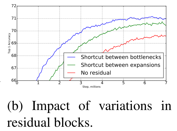
蓝色为逆向残差连接的准确性；
绿色为普通残差连接的准确性；
红色为没有残差连接的准确性；
可以看出，在同等条件下，逆向残差准确性最高；

5.1.2 线性瓶颈

图6(a)：线性瓶颈的影响

蓝色为在bottleneck后使用线性激活的结果；
绿色为在bottleneck后使用非线性激活的结果；
可以看出，同等条件下，使用线性激活准确性高；