[Machine Learning] Neural Network

Neural Network

1. Central idea about neural network

In general, neural network is just a semi-parameter statistical model. The central ideal is to extract linear combinations of inputs as derived features, and then model the target as a nonlinear function of these features. Or from the network diagram view, we can regard neural network as the standard linear model or multilogistic model on the hidden layer.

2. Understanding of neural network

Let’s look at the diagram of neural network.

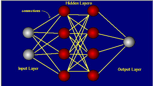
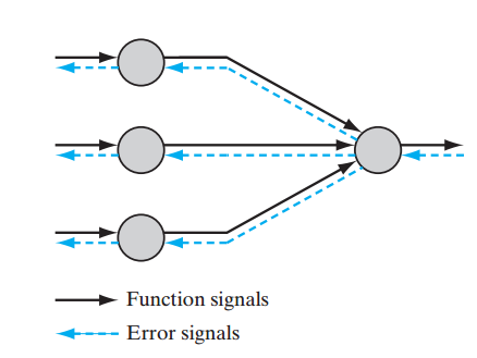
This is a neural network which contains just one hidden layer. You can see that it is a graph with connections only exiting in neighboring layers. And each node is derived via an activation function of linear combinations of nodes in previous layer. To see the mechanism more clearly, look at the following picture

This picture tells us how the node is derived from previous layer.

• firstly, we make a linear combination of all nodes in previous layer via $\omega$ parameters.
  $$v_k = \sum_{i=0}^m\omega_{ki}x_i$$
• then, we use an activation function $\phi$ to give the value of this node.
  $$\hat y_k = \phi(v_k)$$

So, putting them together, we get the formula of it

$$\hat y_k = \phi\left(\sum_{i=0}^m\omega_i x_i\right)$$
which can be viewed as one-dimensional Projection Pursuit Method.

3. Back-Propagation algorithm

To determine the parameters used in neural network, measures of fit are needed be to set up.

Notations used: $\theta$ contains all parameters in all layers; $N$ means the number of training data

• for regression, RSS(residual sum of square) is used.
  $$R(\theta) = \frac{1}{2}\sum_{i=1}^N\sum_{k=1}^K(y_{ik}- \hat y_{ik})^2\underbrace{+\lambda\|\theta\|_2^2}_{\text{weight decay}}$$
  • for classification, cross-entropy is used.
    $$R(\theta) = - \sum_{i=1}^N\sum_{k=1}^K y_{ik}\log (\hat y_{ik})\underbrace{+\lambda\|\theta\|_2^2}_{\text{weight decay}}$$

  • The function of the weight decay item can avoid overfit problem. And minimizing $R(\theta)$ always use gradient descent, called back-propagation in this setting. Why this name is called will be clear after reading following section.

    Consider neural network containing only one hidden layer as example (with $\alpha$, $\beta$ denoting as the parameters of first and second layers) and take RSS as error measure, then we derive the formula for back-propagation algorithm. We have
    

    $$R(\theta) = \sum_{i=1}^N R_i(\theta) +\lambda\|\theta\|_2^2= \frac{1}{2}\sum_{i=1}^N\sum_{k=1}^K (y_{ik}- \hat y_{ik})^2+\lambda\|\theta\|_2^2$$

    If we derive the derivatives of $\alpha$ and $\beta$, we have
    

    $$\frac{\partial R_i}{\partial \beta_{km}} = \delta_{ki} x^{(2)}_{mi}$$
    $$\frac{\partial R_i}{\partial \alpha_{ml}} = s_{mi} x^{(1)}_{il}$$
    with
    $$s_{mi} = \gamma(\theta)\delta_{ki}$$

    So error term $s_{ml}$ in updating parameters in the first layer bases on the error term $\delta_{ki}$ in updating parameters in the latter layer. From that we can see that

    • the direction of prediction is from the lower layer to the upper.
    • the direction of updating parameters in gradient descent algorithm is form the upper layer to the lower.

    This is why we call the gradient descent as back-propagation algorithm.

    

    The advantage of back-propagation are its simple, local nature. In the pack-propagation algorithm, each hidden unit passes and receives information only to and from units that share a connection. Hence it can be implemented efficiently on a parallel architecture computer.—-‘Element of Statistical Learning’

    4. Situations neural network to be used

    Since features used in neural network are so complex, the neural network is not very useful for understanding the importance of features and is little interpretable. But in return, due to its complexity, it can capture the nonlinearity of hidden model. So neural network has great performance of prediction.

    Neural network is especially effective in problems with a high signal-to-noise ratio and settings where prediction without interpretation is the goal. It is less effective for problems where the goal is to describe the physical process that generated the data and the roles of individual inputs.