第十章 曲线拟合

目录：
1.线性函数拟合
2.指数函数的拟合

1.线性函数拟合

线性函数很好描述的一个数集：

y = mx + b

（1）输入数据

handicap = [6:2:24]

6 8 10 12 14 16 18 20 22 24

Ave = [3.94, 3.8, 4.1, 3.87, 4.45, 4.33, 4.12, 4.43, 4.6, 4.5];

（2）求解系数

p = polyfit(handicap,Ave,1);产生一个1阶多项式系数

（3）系数配置

m = p(1)

m = 0.0392

b = p(2)

b = 3.6267

（4）产生一个函数绘出 y = mx + b 的直线

x = [6:0.1:24];//建立x轴

y = m*x + b;//产生直线

（5）绘图

subplot(2,1,2);绘图框设置

plot(handicap,Ave,‘o’,x,y),xlabel(‘差点’),ylabel(‘平均成绩’)//绘制直线并圈出实际数据

w = m*handicap + b

w =

Columns 1 through through 10

3.8616 3.9399 4.0182 4.0965 4.1748 4.2532 4.3315 4.4098 4.4881 4.5664

（6）计算误差来评估拟合程度

r2 = 1 - A/S(拟合程度公式）

N = 10; 183

MEAN = sum(Ave)/N//平均值计算

MEAN = 4.2140

mean(Ave)//平均值计算

ans = 4.2140

S = sum((Ave - MEAN).^2)

S = 0.7332

A = sum((w - Ave).^2)

A = 0.2274

r2 = 1 - A/S

r2 = 0.6899

（7）均方根（Root-Mean-Square，RMS）误差

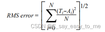
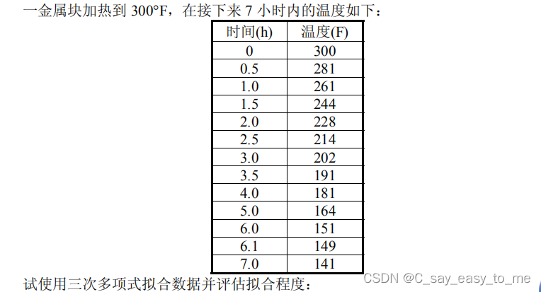
time = [0,0.5,1.0,1.5,2,2.5,3,3.5,4,5,6,6.1,7];横坐标数据输入

temp = [300,281,261,244,228,214,202,191,181,164,151,149,141];纵坐标数据输入

subplot(2,1,1), plot(time,temp,‘o’),xlabel(‘时间（h）’), …

ylabel(‘温度（F）’),title(‘冷却块的温度’);//绘图

p = polyfit(time,temp,3);//产生三阶多项式参数

拟合函数具有下面的形式：y = p1x + p2x + p3x + p4

a = p(1); b = p(2); c = p(3); d = p(4);

t = linspace(0,7);//创建x轴

y = at.^3 + bt.^2 + c*t + d;//定义拟合函数

w = atime.^3 + btime.^2 + c*time + d;//实际温度数值

plot(time,temp,‘o’,t,y),xlabel(‘时间(h)’), …

ylabel(‘温度(F)’),title(‘冷却金属块的三阶拟合图象’)

M1 = mean(temp)//平均值计算

M1 = 208.2308

S = sum((temp - M1).^2)//

S = 3.2542e+004

A = sum((w-temp).^2)

A = 2.7933

r2 = 1 - A/S//求得拟合程度

r2 = 0.9999

format long

r2

r2 =0.99991416476050

N = 13;

RMS = sqrt(sum((1/N)*(w-temp).^2))//求得RMS误差

RMS = 0.46353796413735

t = [0:0.1:15];//延伸时间线

y = at.^3 + bt.^2 + c*t + d;//重新拟合多项式

find(y < 80)//查找y小于80度的x值

ans = 148 149 150 151

format short//数据格式改为短整型

A = t(148:151)’

A =

14.7000

14.8000

14.9000

15.0000

B = y(148:151)’

B =

78.5228

77.0074

75.4535

73.8604

Table = [A B]//将A，B矩阵组合成增广矩阵

Table =

14.7000 78.5228

14.8000 77.0074

14.9000 75.4535

15.0000 73.8604

2.指数函数的拟合

拟合推导：

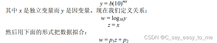
p = polyfit(x, log10(y), 1)//产生参数

m = p , b = p2//参数配置