《统计学习方法》—— 2. 感知器（Python实现）

本文完整代码 github 地址：https://github.com/anlongstory/awsome-ML-DL-leaning/lihang-reading_notes ( 如果觉得不错，欢迎 Star ?)

本文主要是在阅读过程中对本书的一些概念摘录，包括一些个人的理解，主要是思想理解不涉及到复杂的公式推导。若有不准确的地方，欢迎留言指正交流

感知器

感知机(perceptron) 是而二分类的线性分类模型，输入为特征向量，输出为类别取，+1，-1二值。用函数式来表达就是下面的公式：

f(x) = sign (w*x + b)

 其中 w 称为权重（weight）， b 叫做偏置（bias）。

对应理解就是在特征空间 Rⁿ中的一个超平面，w 是超平面的法向量， b 是超平面的截距。

感知器学习策略

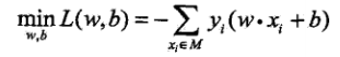
感知器学习的策略是极小化损失函数：

损失函数对应的是误分类点到分类超平面的总距离。其中 y _i 只有 +1，或 -1，当 w\*x _i + b > 0 时， y _i = 1 ，反之 w\*x _i + b < 0 时， y _i = -1 。所以 -y _i（w\*x _i + b）> 0 时，w\*x _i + b > 0 时， y _i = -1，反之为正 1，可以表示误分类点到超平面的距离。

感知器学习算法

感知器学习算法是基于随机梯度下降法的对损失函数的最优化算法，有原始形式和对偶形式两种。

• 原始形式

   学习过程：

w = w + ηy_ix_i
b = b + ηy_i

• 对偶形式
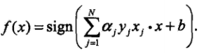
  感知器模型为：

   学习过程：

α_i = α_i + η
b = b + ηy_i

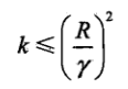
当训练集线性可分时，感知器学习算法是收敛的。感知器计算在训练数据集上的误分类次数 k 满足不等式：

其中，R 是所有特征向量 x _i 中的最大模，γ 为当前所有特征向量 x _i 分别代入超平面方程中的最小值。

当训练集线性可分时，感知器学习算法存在无穷多个解，其解由于不同的初值或不同的迭代顺序而可能不同。

代码实现

感知器示例代码：

from sklearn.linear_model import Perceptron
import matplotlib.pyplot as plt
import pandas as pd
import numpy as np
from sklearn.datasets import load_iris

# 数据集准备
iris = load_iris()
df = pd.DataFrame(iris.data, columns=iris.feature_names)
df['label'] = iris.target
data = np.array(df.iloc[:100, [0, 1, -1]])
X, y = data[:,:-1], data[:,-1]
y = np.array([1 if i == 1 else -1 for i in y])


# part 1 感知器模型
class Model:
    def __init__(self):
        self.w = np.ones(len(data[0]) - 1, dtype=np.float32)
        self.b = 0
        self.l_rate = 0.1
        # self.data = data

    def sign(self, x, w, b):
        y = np.dot(x, w) + b
        return y

    # 随机梯度下降法
    def fit(self, X_train, y_train):
        is_wrong = False
        while not is_wrong:
            wrong_count = 0
            for d in range(len(X_train)):
                X = X_train[d]
                y = y_train[d]
                if y * self.sign(X, self.w, self.b) <= 0:
                    self.w = self.w + self.l_rate * np.dot(y, X)
                    self.b = self.b + self.l_rate * y
                    wrong_count += 1
            if wrong_count == 0:
                is_wrong = True
        return 'Perceptron Model!'

perceptron = Model()
perceptron.fit(X, y)
x_points = np.linspace(4,7,10)
y_ = -(perceptron.w[0]*x_points + perceptron.b)/perceptron.w[1]


# part 2 scikit-learn 实现
# clf = Perceptron(fit_intercept=False, max_iter=1000, shuffle=False)
# clf.fit(X, y)
#
# x_points = np.arange(4, 8)
# y_ = -(clf.coef_[0][0]*x_points + clf.intercept_)/clf.coef_[0][1]



plt.plot(x_points, y_)
plt.plot(data[:50, 0], data[:50, 1], 'bo', color='blue', label='0')
plt.plot(data[50:100, 0], data[50:100, 1], 'bo', color='orange', label='1')
plt.xlabel('sepal length')
plt.ylabel('sepal width')
plt.legend()
plt.show()

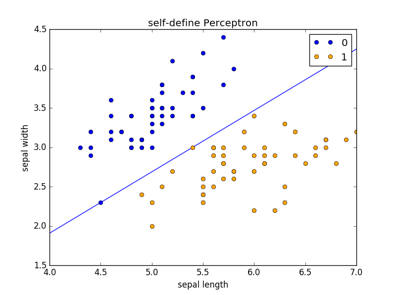
运行完 part 1 结果为：

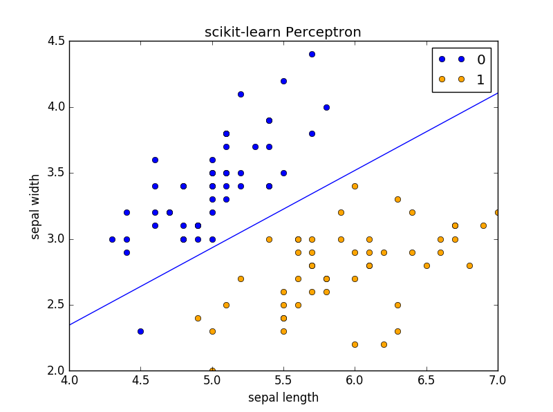
也可以将part 1 感知器模型 部分注释，将 part 2 scikit-learn 实现 解注释，运行，运行完 part 2 结果为：

相关阅读：

《统计学习方法》—— 1. 统计学习方法概论（Python实现）
《统计学习方法》—— 3. K近邻法（Python实现）
《统计学习方法》—— 4. 朴素贝叶斯（Python实现）
《统计学习方法》—— 5. 决策树（Python实现）
《统计学习方法》—— 6. 逻辑斯特回归与最大熵模型（Python实现）
《统计学习方法》—— 7. 支持向量机（Python实现）
《统计学习方法》—— 8. 提升方法 （Python实现）
《统计学习方法》—— 9. EM 算法（Python实现）
《统计学习方法》——10. 隐马尔可夫模型（Python实现）
《统计学习方法》—— 11. 条件随机场