Faster-RCNN论文及原码解读

论文： 链接
原码： 链接

一、模型的整体框架

从上图可以看出，算法整体可以分为四个阶段：
1、conv layers：提取特征图，Faster-RCNN首先用一组基础的网络结构conv+relu+pooling层来提取input image的feature maps，提取出的feature map用于后续的RPN和ROI Pooling。例如backbone网络为VGG16，网络结构为13个conv+13个relu+4个pooling层组成。

2、Region Proposal Network：RPN网络主要用于生成region proposals，首先生成一堆的anchor，然后对其进行裁剪过滤通过softmax判断anchors是属于前景（foreground）还是后景（background），即是物体or不是物体，所以这是一个二分类；同时，另一支bounding box regression修正anchor box，形成较为精确的proposal。

3、ROI Pooling：利用RPN生成的proposals和backbone网络最后一层得到的feature map，得到固定大小的proposal feature map，进入后面的全连接层进行目标的识别和定位。

4、Classifer：将ROI Pooling层形成固定大小的feature map进行全连接操作，利用softmax进行具体类别的分类，同时，利用L1 Loss完成bounding box 回归操作获得物体的精确定位。

二、网络结构

2.1 Conv Layers

【Faster-rcnn读取图像尺寸问题】
Faster rcnn一般对输入图像的大小尺寸限制为：最小边为600，最大边为1000，
假定输入图像尺寸为：H×W

【backbone 结构】
以VGG16为例：
13个conv：kernel_size = 3, padding = 1, stride = 1;（经过卷积层，图片的尺寸大小不变）
+
13个relu：激活函数，不改变图片的大小；
+
4个pooling：kernel_size = 2,stride = 2；pooling层会让图片的尺寸变为原来的1/2。

经过conv layer图片的尺寸变为（H/16）*（W/16），即M×N，输出的feature map的大小为M×N×512-d（注：VGG是512-d，ZF是256-d）表示特征图的大小为M×N，维度即数量是512.

2.2 RPN(Region Proposal Networks)

RPN主要分为两路：
rpn_cls和rpn_bbox
feature map进入RPN网络后，先经过一次3×3的卷积，同样，特征图的大小依然是M×N×512，这样做的目的是进一步集中特征信息，接着分两支分别进行两个1×1的卷积，即kernel_size=1,padding=0,stride=1,一支是18-d，一支是36-d。

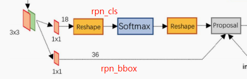
1）rpn_cls:
M×N×512 * 1×1×512×18 -> M×N×18
2）rpn_bbox:
M×N×512 * 1×1×512×36 ->M×N×36

2.2.1 Anchors box的生成

图片经过Conv Layers变为原来的1/16，令feat_stride=16,在生成anchor时，先定义一个base anchor，大小为16×16的box（feature map上的一个点的感受野对应原始图像上是一块区域，这里设置16，是因为feature map上的一点对应原始图像16×16大小的区域），源码转化为[0, 0, 15, 15]的数组，然后设置长宽比和面积比分别是[1:2, 1:1, 2:1]，这样一个box通过这种比例就可以生成9个box。
（源码中的generate_anchors.py）
1、设置base anchor的大小：

base_anchor = np.array([1, 1, base_size, base_size]) - 1
# base_size=16
# base_anchor = [0, 0, 15, 15]

2、base_anchor=[0, 0, 15, 15],面积保持不变，长、宽比分别是[0.5, 1, 2]时产生的anchor

def _ratio_enum(anchor, ratios):
    """
    Enumerate a set of anchors for each aspect ratio wrt an anchor.
    """
    w, h, x_ctr, y_ctr = _whctrs(anchor)
    size = w * h                 # size=16×16=256
    size_ratios = size / ratios  # size_ratios:[512, 256, 128]
    # np.round(x)返回x的四舍五入数字，np.sqrt(x)返回数字x的平方根
    ws = np.round(np.sqrt(size_ratios))  # ws=[23, 16, 11]
    hs = np.round(ws * ratios)           # hs=[12, 16, 22]
    # 转化为anchor的四个坐标值形式
    anchors = _mkanchors(ws, hs, x_ctr, y_ctr)
    return anchors

def _whctrs(anchor):
    """
    Return width, height, x center, and y center for an anchor (window).
    """

    w = anchor[2] - anchor[0] + 1       # xmax - xmin + 1
    h = anchor[3] - anchor[1] + 1       # ymax - ymin + 1
    x_ctr = anchor[0] + 0.5 * (w - 1)   # x_center
    y_ctr = anchor[1] + 0.5 * (h - 1)   # y_center
    return w, h, x_ctr, y_ctr

def _mkanchors(ws, hs, x_ctr, y_ctr):
    """
    Given a vector of widths (ws) and heights (hs) around a center
    (x_ctr, y_ctr), output a set of anchors (windows).
   """

    ws = ws[:, np.newaxis]
    hs = hs[:, np.newaxis]
    anchors = np.hstack((x_ctr - 0.5 * (ws - 1), y_ctr - 0.5 * (hs - 1),
                         x_ctr + 0.5 * (ws - 1), y_ctr + 0.5 * (hs - 1)))
    return anchors

生成的anchor为：

array([[-3.5,  2. , 18.5, 13. ],
       [ 0. ,  0. , 15. , 15. ],
       [ 2.5, -3. , 12.5, 18. ]])

3、经过上面的长宽比变换之后，接下来执行的是面积scales的变换：

# scales = 2 ** np.arange(3, 6) = [8, 16, 32]
anchors = np.vstack([
        _scale_enum(ratio_anchors[i, :], scales) for i in range(ratio_anchors.shape[0])
        ])

上面的_scale_enum()函数的定义如下，对上一步得到的ratio_anchors中的三种宽高比的anchor，再分别进行三种scale的变换，也就是三种宽高比，搭配三种scale，最终会得到9种宽高比和scale 的anchors。这就是论文中每一个点对应的9种anchors。

def _scale_enum(anchor, scales):
    """
    Enumerate a set of anchors for each scale wrt an anchor.
    """
    w, h, x_ctr, y_ctr = _whctrs(anchor)
    ws = w * scales
    hs = h * scales
    anchors = _mkanchors(ws, hs, x_ctr, y_ctr)
    return anchors

_scale_enum函数中也是首先将宽高比变换后的每一个ratio_anchor转化成（宽，高，中心点横坐标，中心点纵坐标）的形式，再对宽和高均进行scale倍的放大，然后再转换成四个坐标值的形式。最终经过宽高比和scale变换得到的9种尺寸的anchors的坐标如下：

array([[ -83.,  -39.,  100.,   56.],
      [-175.,  -87.,  192.,  104.],
      [-359., -183.,  376.,  200.],
      [ -55.,  -55.,   72.,   72.],
      [-119., -119.,  136.,  136.],
      [-247., -247.,  264.,  264.],
      [ -35.,  -79.,   52.,   96.],
      [ -79., -167.,   96.,  184.],
      [-167., -343.,  184.,  360.]])

图片显示这9个anchor如下：

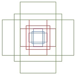
上面描述了feature map上的一个点生成9个anchor的过程，对feature map上的每一个点都要生成9个anchor，即要生成M×N×9个anchor。（源码对应snippets.py）

def generate_anchors_pre(height,
                         width,
                         feat_stride,
                         anchor_scales=(8, 16, 32),
                         anchor_ratios=(0.5, 1, 2)):
    """ 
    A wrapper function to generate anchors given different scales
    Also return the number of anchors in variable 'length'
    """
    # 生成长宽比和面积比不同的9个anchor
    anchors = generate_anchors(
        ratios=np.array(anchor_ratios), scales=np.array(anchor_scales))
    # A = 9
    A = anchors.shape[0]
    # 横向偏移量（0，16，32，...）
    shift_x = np.arange(0, width) * feat_stride
    # 纵向偏移量（0，16，32，...）
    shift_y = np.arange(0, height) * feat_stride
    
    """
    shift_x = [[0，16，32，..],[0，16，32，..],[0，16，32，..]...],
    shift_y = [[0，0，0，..],[16，16，16，..],[32，32，32，..]...],
    就是形成了一个纵横向偏移量的矩阵，也就是特征图的每一点都能够通过这个
    矩阵找到映射在原图中的具体位置！
    """
    shift_x, shift_y = np.meshgrid(shift_x, shift_y)
    """
    经过刚才的变化，其实大shift_x, shift_y的元素个数已经相同，看矩阵的结构也能看出，
    矩阵大小是相同的，sift_x.ravel()之后变成一行，此时shift_x,shift_y的元
    素个数是相同的，都等于特征图的长宽的乘积(像素点个数)，不同的是此时
    的shift_x里面装得是横向看的x的一行一行的偏移坐标，而此时的y里面装
    的是对应的纵向的偏移坐标！
    """
    # shift_x.ravel():(M×N,) shift_y.ravel():(M×N,)
    # transpose:(4, M×N) -> (M×N, 4)
    shifts = np.vstack((shift_x.ravel(), shift_y.ravel(), shift_x.ravel(),
                        shift_y.ravel())).transpose()

    # 读取特征图中元素的总个数
    K = shifts.shape[0]
    """
    width changes faster, so here it is H, W, C
    用基础的9个anchor的坐标分别和偏移量相加，最后得出了所有的anchor的坐标，
    四列可以堪称是左上角的坐标和右下角的坐标加偏移量的同步执行，飞速的从
    上往下捋一遍，所有的anchor就都出来了！一共K个特征点，每一个有A(9)个
    基本的anchor，所以最后reshape((K*A),4)的形式，也就得到了最后的所有
    的anchor左下角和右上角坐标.
    """
    anchors = anchors.reshape((1, A, 4)) + shifts.reshape((1, K, 4)).transpose((1, 0, 2))
    anchors = anchors.reshape((K * A, 4)).astype(np.float32, copy=False)  
    length = np.int32(anchors.shape[0])

    return anchors, length

特征图的大小是M×N，所以一共生成M×N×9个anchor box

【总结：从9个base anchor 如何生成M×N×9个anchor】
通过width：(0-60)*16, height:(0-40)*16, 建立shift偏移量数组，再和base_anchor的基准数组累加，得到特征图上所有像素对应的anchor的坐标值，是一个[K * A, 4]数组。

以上生成anchor box的过程可总结如下：

2.2.2 RPN实现原理

caffe版本的网络模型结构：

rpn网络结构的实现：(源码对应network.py)

# 以feature map:[1, 1024, 29, 63]为例
def _region_proposal(self, net_conv):

    # *************分类网络：判断前景还是背景*************
    # feature map:net_conv
    # self.rpn_net:Conv2d(1024, 512, kernel_size=[3, 3], stride=(1, 1), padding=(1, 1))
    # rpn:[1, 1024, 29, 63] -> [1, 512, 29, 63]
    rpn = F.relu(self.rpn_net(net_conv))
    self._act_summaries['rpn'] = rpn

    # self.rpn_cls_score_net:Conv2d(521, 18, kernel_size=[1, 1], stride=(1,1))
    # rpn_cls_score:[1, 18, 29, 63]
    rpn_cls_score = self.rpn_cls_score_net(rpn)  # batch * (num_anchors * 2) * h * w

    # change it so that the score has 2 as its channel size
    # rpn_cls_score_reshape:[1, 2, 9×29, 63]
    rpn_cls_score_reshape = rpn_cls_score.view(1, 2, -1, rpn_cls_score.size()[-1])  # batch * 2 * (num_anchors*h) * w
    # rpn_cls_prob_reshape:[1, 2, 9×29, 63]
    rpn_cls_prob_reshape = F.softmax(rpn_cls_score_reshape, dim=1)

    # Move channel to the last dimenstion, to fit the input of python functions
    # rpn_cls_prob:[1, 29, 63, 18]
    rpn_cls_prob = rpn_cls_prob_reshape.view_as(rpn_cls_score).permute(0, 2, 3, 1)  # batch * h * w * (num_anchors * 2)
    # rpn_cls_score:[1, 29, 63, 18]
    rpn_cls_score = rpn_cls_score.permute(0, 2, 3,