Frequency Filters-1

Some basic knowledge about the filtering in frequency domain, all concluded from the book “Digital Image Processing”

1. The 1-D discrete Fourier transform (DFT) is,

$$F(u)=\sum^{M-1}_{x=0}f(x)e^{-j2\pi ux/M},u=0,1,2,...,M-1$$
and the inverse discrete Fourier transform (IDFT) is,
$$f(x)=\frac{1}{M}\sum^{M-1}_{u=0}F(u)e^{j2\pi ux/M},x=0,1,2,...,M-1$$
It indicates that, for each frequency $u$, all discrete variable $x$ are needed for computing the Fourier transform, just with the difference in exponential term.

---

2. Both the DFT and IDFT are infinitely periodic, with period $M$. That is,

$$F(u)=F(u+kM),f(x)=f(x+kM)$$
where k is an integer.

---

3. The 2-D discrete Fourier transform is,

$$F(u,v)=\sum_{x=0}^{M-1}\sum_{y=0}^{N-1}f(x,y)e^{-j2\pi (ux/M+vy/N)}$$
where, $u=0,1,2,...,M-1; v=0,1,2,...,N-1$
and the inverse discrete Fourier transform is,
$$f(x,y)=\frac{1}{MN}\sum_{u=0}^{M-1}\sum_{v=0}^{N-1}F(u,v)e^{j2\pi (ux/M+vy/N)}$$
for $x=0,1,2,...,M-1; y=0,1,2,...,N-1$

---

4. As in 1-D case, the 2-D Fourier transform and its inverse are infinitely periodic in the $u$ and $v$ directions, that is,

$$F(u,v)=F(u+k_1M,v)=F(u,v+k_2N)=F(u+k_1M,v+k_2N)$$
$$f(x,y)=f(x+k_1M,y)=f(x,y+k_2N)=f(x+k_1M,y+k_2N)$$
where $k_1$ and $k_2$ are integers.

---

5. Fourier transform pair satisfies the following translation and rotation properties,

$$f(x,y)e^{j2\pi (u_0x/M+v_0y/N)} \Leftrightarrow F(u-u_0,v-v_0)$$
$$f(x-x_0,y-y_0)=F(u,v)e^{-j2\pi (ux_0/M+vy_0/N)}$$
the first equation means, multiplying $f(x,y)$ by the exponential shown shifts the origin of the DFT to $(u_0,v_0)$ and, conversely, multiplying $F(u,v)$ by the negative of that exponential shifts the origin of $f(x,y)$ to $(x_0,y_0)$.

Besides the translation cases, the Fourier transform pairs also has the following property,

$$f(r,\theta+\theta_0) \Leftrightarrow F(\omega,\varphi+\theta_0)$$
here using the polar coordinates,
$$x=rcos\theta,y=rsin\theta,u=\omega cos\varphi,v=\omega sin\varphi$$
that indicates that rotating $f(x,y)$ by an angle $\theta_0$ rotates $F(u,v)$ by the same angle.Conversely, rotating $F(u,v)$ rotates $f(x,y)$ by the same angle.

The translation property is very useful,
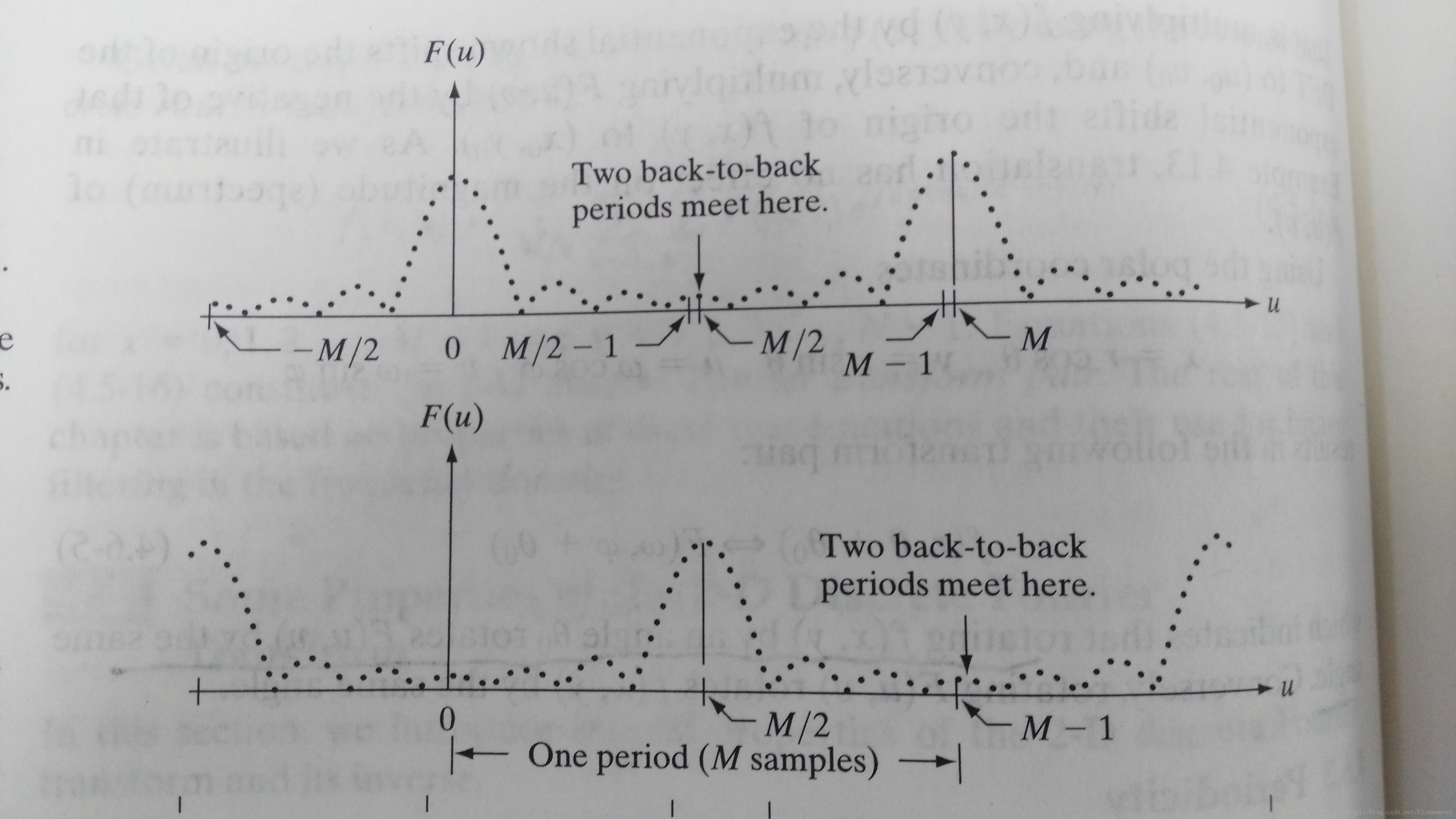
Consider the 1-D spectrum in the below Figure, the transform data in the interval from 0 to $M-1$ consists of two back-to-back half periods meeting at the point $M/2$. For display and filtering purposes, it is more convenient to have in this interval a complete period of the transform in which the data are contiguous with the aid of below equation,

$$f(x)e^{j2\pi (u_0x/M)} \Leftrightarrow F(u-u_0)$$
if we set $u_0=M/2$, the exponential term will be $(-1)^x$, and the Fourier form will shift $M/2$, that is,
$$f(x)(-1)^x \Leftrightarrow F(u-M/2)$$
so, the $F(0)$ is at the center of the interval $[0,M-1]$

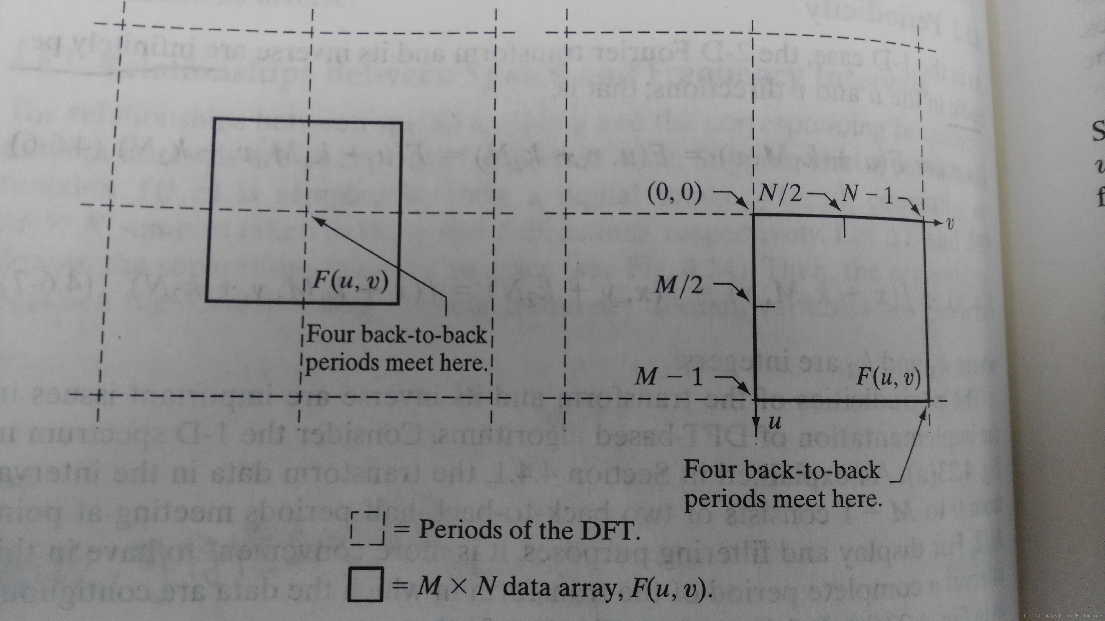
Consider the same way in 2-D case, multiply the exponential term with the original digital image data $f(x,y)$ will shift the Fourier Form $F(0,0)$ at $(M/2,N/2)$, the center of the intervals $[0,M-1]$ and $[0,N-1]$, as shown below.

$$f(x,y)(-1)^{x+y} \Leftrightarrow F(u-M/2,v-N/2)$$

---

6. In fact, the DFT is a complex , which is consist of real part and imaginary part. the magnitude of the DFT is called the Fourier spectrum,

$$|F(u,v)|=[R^2(u,v)+I^2(u,v)]^{\frac{1}{2}}$$
and
$$\phi(u,v)=arctan[\frac{I(u,v)}{R(u,v)}]$$
is called the phase angle.
where the $R$ and $I$ are the real and imaginary parts of $F(u,v)$, the spectrum and phase are all $M*N$ array.

---

7. It’s clear from the Fourier equation that,

$$F(0,0)=\sum_{x=0}^{M-1}\sum_{y=0}^{N-1}f(x,y)$$
which indicates that the zero-frequency term is proportional to the average value of $f(x,y)$, that is,
$$F(0,0)=MN\frac{1}{MN}\sum_{x=0}^{M-1}\sum_{y=0}^{N-1}f(x,y)=MN\overline f(x,y)$$
where $\overline f(x,y)$denotes the average value of $f$. Sometimes, $F(0,0)$ is called the DC component of the transform.

---

8. The 2-D DFT is separable into 1-D transforms,

$$F(u,v)=\sum_{x=0}^{M-1}e^{-j2\pi ux/M}\sum_{y=0}^{N-1}e^{-j2\pi vy/N}=\sum_{x=0}^{M-1}F(x,v)e^{-j2\pi ux/M}$$
where,
$$F(x,v)=\sum_{y=0}^{N-1}f(x,y)e^{-j2\pi vy/N}$$
We can see, $F(x,v)$ is simply the 1-D DFT of a row of $f(x,y)$. By varying $x$ from 0 to M-1, we compute a set of 1-D DFTs for all rows of $f(x,y)$. Thus, we conclude that the 2-D DFT of $f(x,y)$ can be obtained by computing the 1-D transform of each row of $f(x,y)$ and then computing the 1-D transform along each column of the result.

---

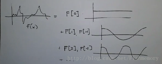
9. Actually, the 2-D DFT is like a decomposition of an image into complex exponential (i.e. sines and cosines)

$$F(u)=\sum^{M-1}_{x=0}f(x)e^{-j2\pi ux/M}=\sum^{M-1}_{x=0}f(x)[cos(\frac{2\pi ux}{M})-jsin(\frac{2\pi ux}{M})],u=0,1,2,...,M-1$$

here is one Fourier transform illustration of random 1-D function $f(x)$, which can be regarded as a series of cosine and sine curves.

---

10. We refer to the domain of $t$ as the spatial domain, and the domain of $\mu$ as the frequency domain, the preceding equation tells us that the Fourier transform of the convolution of two functions in the spatial domain is equal to the product in the frequency domain of the Fourier transforms of the two functions. Conversely, if we have the product of the two transforms, we can obtain the convolution in the spatial domain by computing the inverse Fourier transform. In other words, $f(x)\bigstar g(x)$ and $H(\mu)F(\mu)$ are a Fourier transform pair.

$$f(x)\bigstar g(x) \Leftrightarrow H(\mu)F(\mu)$$

For 1-D case, the discrete equivalent of the convolution is,

$$f(x) \bigstar h(x) =\sum_{m=0}^{M-1} f(m)h(x-m)$$
for $x=0,1,2,...,M-1$, where the minus sign accounts for the flipping, and $x$ is the displacement needed to slide one function past the other.

Here gives one 1-D discrete convolution example, the left column of the below figure implements convolution of two functions, $f$ and $h$, using the above euqation, which because the two functions are of the same size, is written as,

$$f(x) \bigstar h(x) =\sum_{m=0}^{399} f(m)h(x-m)$$

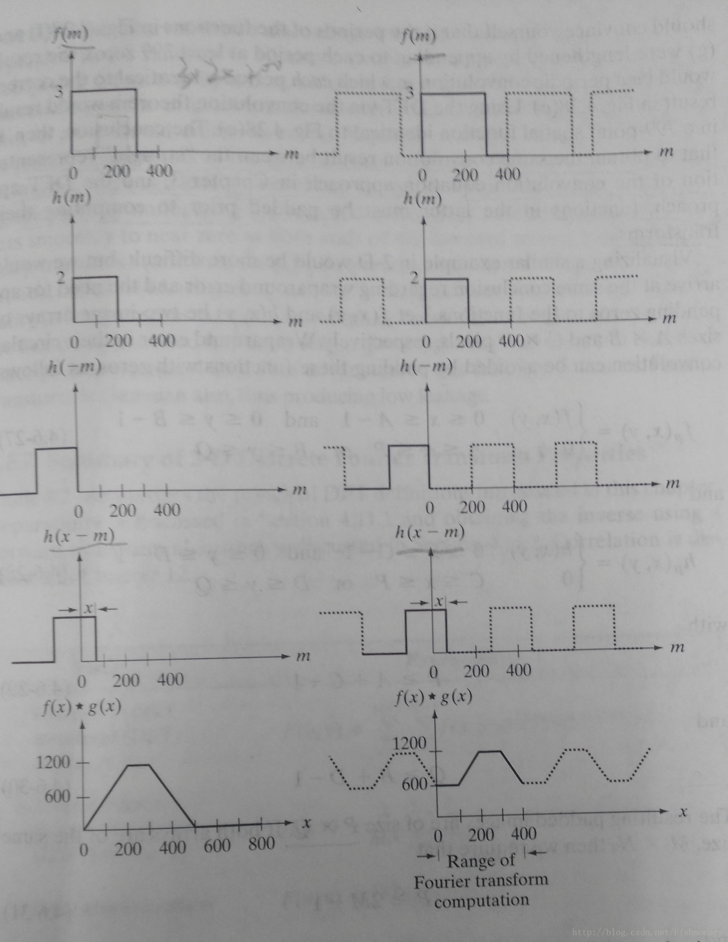
But, one point differs, instead of computing the convolution directly in the spatial domain, if we use the DFT and the convolution theorem to obtain the same result as the left column of the above figure, we must take into account the periodicity inherent in the expression for the DFT. This is equivalent to convolving the two periodic functions in the first two ones on the right column part of the above figure. Proceeding with these two functions will yield the incorrect result, as the last one on the right column part of the figure. The problem stays the two functions interfere with each other to cause what is commonly referred to as wraparound error.
Fortunately, the solution to the wraparound error problem is simple. Consider the two functions $f(x)$ and $h(x)$ composed of A and B samples, respectively. It can be shown that if we append zeros to both functions so that they have the same length, denoted by P, then wraparound is avoided by choosing,

$$P \geq A+B-1$$
This process is called zero padding. In a nut shell, to obtain the same convolution result between the “straight” representation of the convolution equation approach, and the DFT approach, functions must be padded prior to computing their transforms. It is the same in 2-D case, let $f(x,y)$ and $h(x,y)$ be two images arrays of sizes $A*B$ and $C*D$ pixels, respectively, wraparound error in their circular convolution can be avoided by padding these functions with zeros, as follows:
$$f_p(x,y)=\left\{ \begin{aligned} f(x,y) & & 0\leq x \leq A-1&& and &&0\leq y \leq B-1\\ 0 & & A \leq x \leq P&& or &&B \leq y \leq Q \\ \end{aligned} \right.$$

$$h_p(x,y)=\left\{ \begin{aligned} h(x,y) & & 0\leq x \leq C-1&& and &&0\leq y \leq D-1\\ 0 & & C \leq x \leq P&& or &&D \leq y \leq Q \\ \end{aligned} \right.$$
with
$$p \geq A+C-1, Q \geq B+D-1$$