


第一部分:原理详解
目标检测之YOLO算法:YOLOv1,YOLOv2,YOLOv3,TinyYOLO,YOLOv4,YOLOv5,YOLObile,YOLOF,YOLOX详解
目标检测比赛中的tricks(已更新更多代码解析)
【目标检测】YOLO系列总结
一小时内玩转YOLOX(B站视频)
YOLOX-创新点原理、代码精讲(B站视频)(非常好)
第二部分:实验细节记录
YOLOX
零、环境配置
git clone git@github.com:Megvii-BaseDetection/YOLOX.git
cd YOLOX
pip3 install -v -e .  # or  python3 setup.py develop
……
安装apex
下载apex,下载地址,把项目git clone下来,然后
cd path/to/your/apex
python3 setup.py install
安装成功后会显示

参考链接:YOLOX环境搭建
一、Demo,跑通程序
0.首先配置环境
(一)demo.py
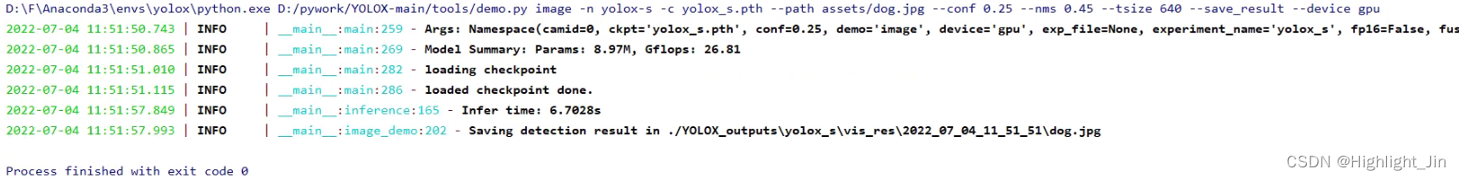
1.首先进行一下测试,通过如下命令。命令行的参数含义:具体参考源码中tools/demo.py中的参数解释
python tools/demo.py image -n yolox-s -c yolox_s.pth --path assets/dog.jpg --conf 0.25 --nms 0.45 --tsize 640 --save_result --device gpu
image表示此处测试的是一张图片;-n yolox-s指定训练过程的模型名称;-c yolox_s.pth指定预训练权重文件;--path assets/dog.jpg测试图片或视频的路径;--conf 0.25画框的阈值;--nms 0.45nms是非极大值抑制的阈值;--tsize 640输入网络图片的尺寸,一般resize成32倍的尺寸,因为图像要进行下采样32倍;--save_result是否保存图片的推理结果,指定后,保存推理的结果。
-b: total batch size, the recommended number for -b is num-gpu * 8
此处补充一张测试成功的截图:
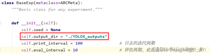
生成的测试结果在如下文件夹下

输出的文件夹目录,若要修改的化是在此处进行修改
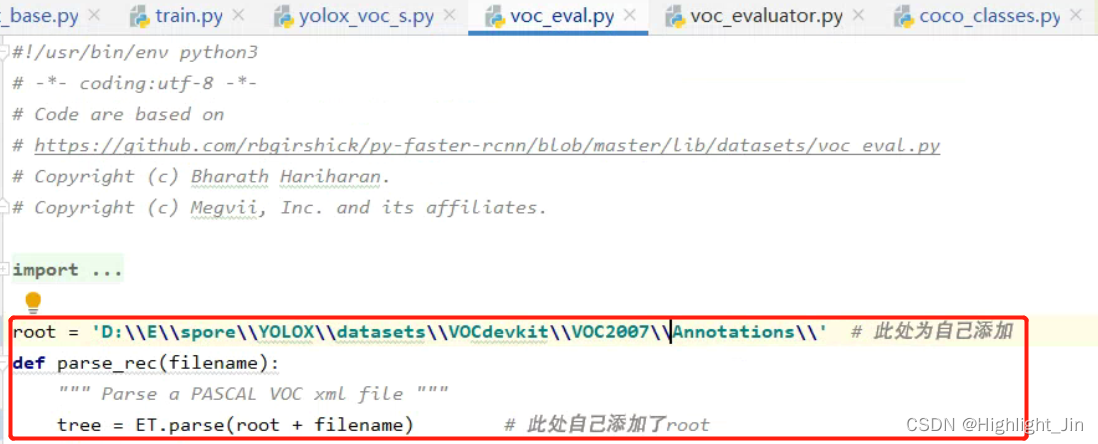
单纯的想用自己的数据测试一下,因为是自定义的数据,coco_classes中已经修改为自己的内容,而这里加载的是官方的预训练权重,所以把coco_classes又改回去。
(二)train.py
2.训练部分
(1)训练命令
python tools/train.py -f D:/pywork/3.debug/YOLOX/exps/example/custom/yolox_s.py -d 1 -b 2
仅指定最简单的参数即可,-f后指定参数文件,-d指定GPU的数量,-b指定batch_size的大小。
(2)加载数据
(2.1)训练过程中指定VOC数据集,则通过-f exps/example/yolox_voc/yolox_voc_s.py指定,完整训练命令,权重的下载地址,指定为自己的路径即可。-d是指定设备的数量,为0和1都是一块GPU(好像是),自己还是指定为了1。-b是指定batch_size的大小。
python tools/train.py -f exps/example/yolox_voc/yolox_voc_s.py -d 1 -b 8 --fp16 -o -c /path/to/yolox_s.pth
python tools/train.py -f exps/example/yolox_voc/yolox_voc_s.py -d 1 -b 8 --fp16 -o -c yolox_s.pth
VOC数据需要解压到datasets中,解压到datasets下之后,文件目录为

自己训练官方voc数据遇到的问题:
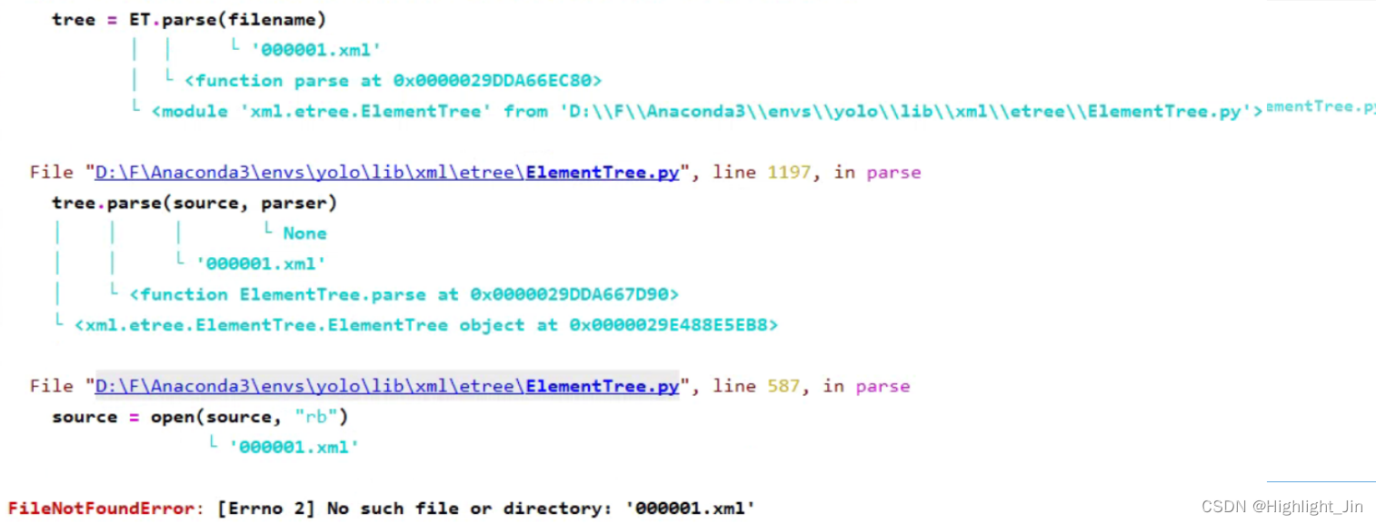
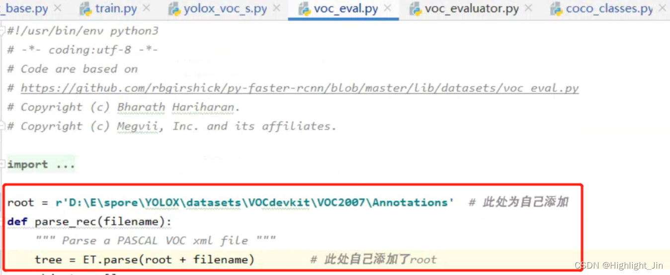
遇到的问题:
1.torch.backends.cudnn.benchmark ?!
RuntimeError: cuDNN error: CUDNN_STATUS_INTERNAL_ERROR
【pytorch】cuDNN error: CUDNN_STATUS_INTERNAL_ERROR终终终终于解决了!
(2.2)训练过程中指定COCO数据集,launch.json文件中参数的指定
"args":[
   "-f", "D:\\E\\spore\\YOLOX\\exps\\example\\custom\\yolox_s.py",//"D:\\E\\spore\\YOLOX\\exps\\default\\yolox_s.py",
   "-d", "1",
   "-b", "8",
   "-c", "D:\\E\\spore\\YOLOX\\yolox_s.pth",
]
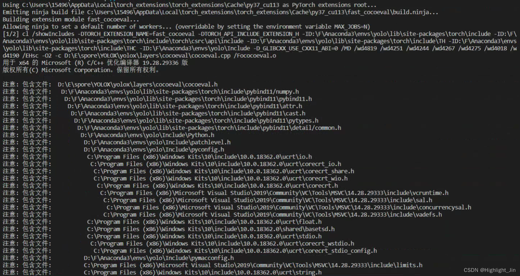
1遇到的问题及解决方案:ModuleNotFoundError: No module named ‘yolox.layers.fast_cocoeval’
from yolox.layers import FastCOCOEvalOp
FastCOCOEvalOp().jit_load()
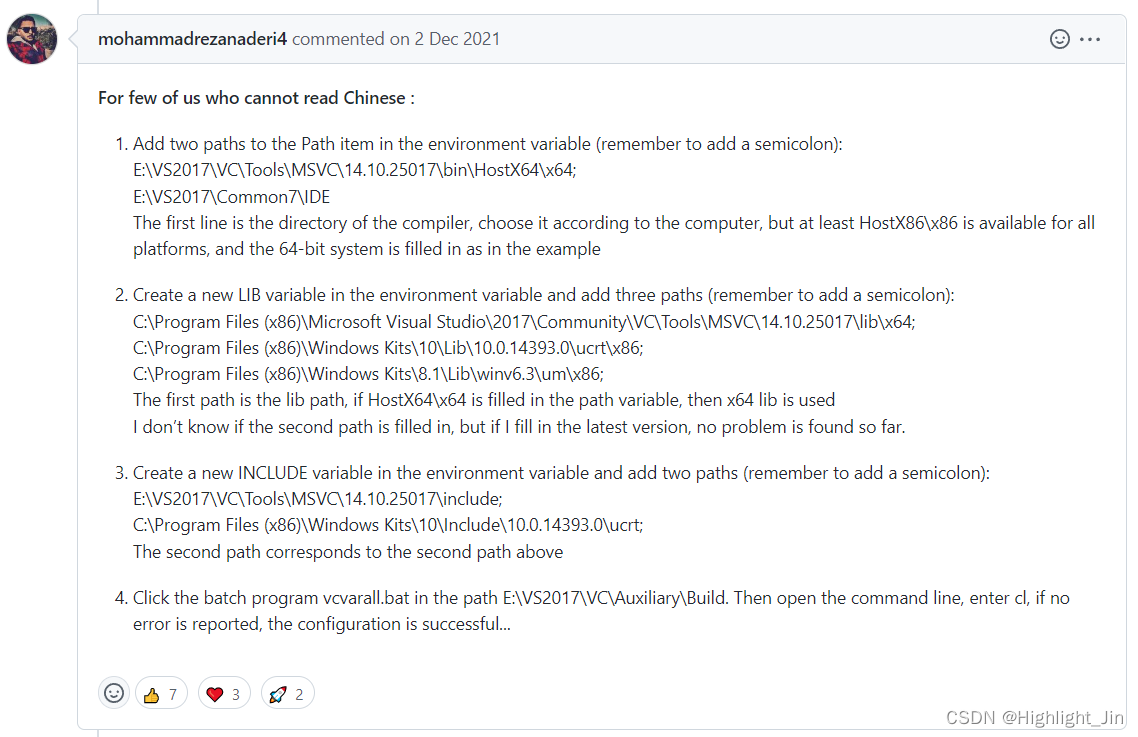
2.又出现新的问题:subprocess.CalledProcessError: Command ‘[‘where’, ‘cl’]’ returned non-zero exit status 1.
解决参考1:官方issue中的代码
解决参考2:subprocess.CalledProcessError: Command ‘[‘where‘, ‘cl‘]‘ returned non-zero exit status 1
答:
自己参考的解决方法:主要参考上面提到的解决参考1
第一步:添加环境变量PATH
C:\Program Files (x86)\Microsoft Visual Studio\2019\Community\VC\Tools\MSVC\14.28.29333\bin\Hostx64\x64
C:\Program Files (x86)\Microsoft Visual Studio\2019\Community\Common7\IDE
第二步:
添加LIB变量,上面截图中这里添加了三个,由于自己没有第三个,所以就没有添加
C:\Program Files (x86)\Microsoft Visual Studio\2019\Community\VC\Tools\MSVC\14.28.29333\lib\x64;
C:\Program Files (x86)\Windows Kits\10\Lib\10.0.18362.0\ucrt\x86;
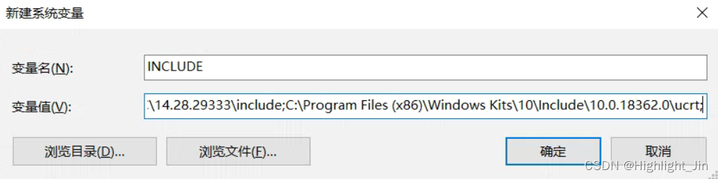
第三步:
添加INCLUDE变量
C:\Program Files (x86)\Microsoft Visual Studio\2019\Community\VC\Tools\MSVC\14.28.29333\include;
C:\Program Files (x86)\Windows Kits\10\Include\10.0.18362.0\ucrt;
上面解决方法图中的第4步自己操作界面一闪而过,所以
进行完第三步之后,自己重新启动了计算机,再次训练代码,终于跑通了。
跑通截图如下:
训练自己的数据集COCO格式步骤简要记录:
1.首先,将自己准备好的数据集放置在如下目录,并按照下面的目录进行命名,这样不用修改项目中的文件名

2.modify exps/example/custom/yolox_s.py as follows:
主要进行了如下修改
3.then, modify the categories in yolox/data/datasets/coco_classes.py
4.modify YOLOX/yolox/exp/yolox_base.py,如有需要进行修改
(三)eval.py
python tools/eval.py -n yolox-s -c yolox_s.pth -b 2 -d 1 --conf 0.001
python -m yolox.tools.eval -n yolox-s -c yolox_s.pth -b 2 -d 1 --conf 0.001
单纯的想用自己的数据测试一下,因为是自定义的数据,coco_classes中已经修改为自己的内容,而这里加载的是官方的预训练权重,所以把coco_classes又改回去。测试demo.py也是同样的操作。测试eval.py脚本,还需要修改一个地方:因为自己定义的数据集中类别数为8,所以在coco.py脚本中self.class_ids = sorted(self.coco.getCatIds())代码生成的结果就是[1,2,3,4,5,6,8]。而本来应该是80类,所以自己在这里手动定义为[1,2,…80]。self.class_ids = list(range(1,81))。之后等自己训练了自己的数据,用自己保存的模型权重进行评估和测试。
二、相关查阅内容
1.Python - 日志管理模块: Loguru的使用(好)
Loguru:优雅的Python程序日志
三、Vscode中launch.json文件参数指定
以下参数全部记录为自己的内容。
{
    // Use IntelliSense to learn about possible attributes.
    // Hover to view descriptions of existing attributes.
    // For more information, visit: https://go.microsoft.com/fwlink/?linkid=830387
    "version": "0.2.0",
    "configurations": [
        {
            "name": "Python: 当前文件",
            "type": "python",
            "request": "launch",
            "program": "${file}",                           // 设置哪个文件为启动文件
            "console": "integratedTerminal",
            "justMyCode": true,
            // "args": ["-f","D:\\E\\spore\\YOLOX\\exps\\example\\yolox_voc\\yolox_voc_s.py", "-d", "0", "-b", "8", "-c", "../yolox_s.pth"]

            // 下面的args是对demo.py进行的参数设置, 可以跑通
            // "args": [
            //     "image",
            //     "-n", "yolox-s",
            //     "-c", "./yolox_s.pth",
            //     "--path", "./assets/dog.jpg",
            //     "--conf", "0.25",
            //     "--nms", "0.60",
            //     "--tsize", "640",
            //     "--save_result",
            //     "--device", "gpu"
            // ],
            // 下面的args是对train.py进行的参数设置,训练的是自己的数据集,已经跑通.起初设置的-d 1 -b 1,测试-b 8可以跑 16也可以跑32不能跑
            // "args":[
            //     "-f", "D:\\E\\spore\\YOLOX\\exps\\example\\custom\\yolox_s.py",//"D:\\E\\spore\\YOLOX\\exps\\default\\yolox_s.py",
            //     "-d", "1",
            //     "-b", "16",
            //     "-c", "D:\\E\\spore\\YOLOX\\yolox_s.pth",
            // ]
            // 下面的args是对eval.py进行的参数设置,对自己的数据集进行评估。
            "args": [
                "-f", "D:\\E\\spore\\YOLOX\\exps\\example\\custom\\yolox_s.py",
                "-d", "1",
                "-b", "16",
            ]
        }
    ]
}
针对train.py脚本中,起初设置的-d 1 -b 1,是为了测试,很快跑通整个流程。然后对batch_size调大-b 8可以跑 16也可以跑32不能跑(3080机器)。
四、数据集的划分
五、loss曲线的绘制
1.YOLOX-绘制五种loss曲线(可直接进行参考,但是总迭代次数iters_num需要自己计算正确)
这里可以绘制loss曲线。
应该是这样计算的:程序中设置每10次迭代,打印一下结果。
首先根据图片总数和batch_size的大小计算1个epoch的迭代次数,比如201张图片,batch_size=8,那么1个epoch就是要迭代26次,每10iter进行一次打印,所以1epoch就打印两条信息。一共300epoch,所以iters_num=300210=600*10 = 6000
2.如何让YOLOX模型evaluation输出漂亮的结果图(这个可参考)
这里可以绘制热力图和P-R图。
有几个关键文件:
- 1.
YOLOX/yolox/evaluators/coco_evaluator.py这是测试主函数, 要在这里调用画图函数和类 - 2.
yolov5/utils/metrics.py这里有所有用到的画图函数和类的本体 - 3.
yolov5/val.py只需要这里的process_batch一个函数, 复制到1.即可
之后,自己对文件目录进行了修改:
(1) 运行train.py修改yolox\core\trainer.py部分
self.evaluator = self.exp.get_evaluator(
            batch_size=self.args.batch_size, is_distributed=self.is_distributed,
            save_dir = self.file_name,      # 这个参数是自己加的
        )
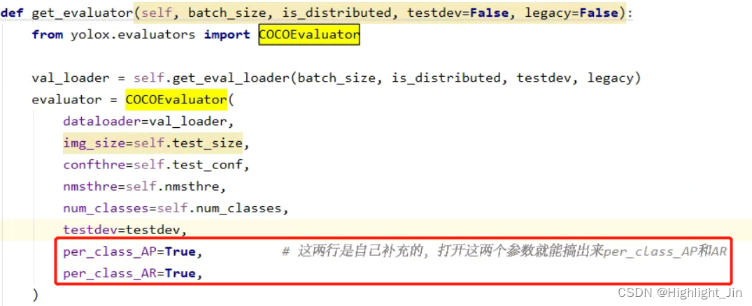
(2)修改yolox\exp\yolox_base.py部分
evaluator = COCOEvaluator(
            dataloader=val_loader,
            img_size=self.test_size,
            confthre=self.test_conf,
            nmsthre=self.nmsthre,
            num_classes=self.num_classes,
            save_dir=save_dir,          # 这行是自己添加
            testdev=testdev,
            per_class_AP=True,          # 这两行是自己补充的,打开这两个参数就能搞出来per_class_AP和AR
            per_class_AR=True,
        )
(3)修改yolox\evaluators\coco_evaluator.py部分
class COCOEvaluator:
    """
    COCO AP Evaluation class.  All the data in the val2017 dataset are processed
    and evaluated by COCO API.
    """

    def __init__(
        self,
        dataloader,
        img_size: int,
        confthre: float,
        nmsthre: float,
        num_classes: int,
        save_dir: str,              # 这行自己添加
        testdev: bool = False,
        per_class_AP: bool = False,
        per_class_AR: bool = False,
    ):
        """
        Args:
            dataloader (Dataloader): evaluate dataloader.
            img_size: image size after preprocess. images are resized
                to squares whose shape is (img_size, img_size).
            confthre: confidence threshold ranging from 0 to 1, which
                is defined in the config file.
            nmsthre: IoU threshold of non-max supression ranging from 0 to 1.
            per_class_AP: Show per class AP during evalution or not. Default to False.
            per_class_AR: Show per class AR during evalution or not. Default to False.
        """
        self.dataloader = dataloader
        self.img_size = img_size
        self.confthre = confthre
        self.nmsthre = nmsthre
        self.num_classes = num_classes
        self.save_dir = save_dir                    # 这行自己添加
        self.testdev = testdev
        self.per_class_AP = per_class_AP
        self.per_class_AR = per_class_AR
(4)主循环前定义变量, COCOEvaluator类的evaluate函数内, for循环前:
# 自己添加
iouv = torch.linspace(0.5, 0.95, 10, device='cpu')
niou = iouv.numel()
confusion_matrix = ConfusionMatrix(nc=self.num_classes)
stats = []
seen = 0
names = ['graminearum', 'avenaceum', 'culmorum', 'moniliforme',
       'doutan', 'jujiao', 'putao', 'liangsan']  # 类名
names_dic = dict(enumerate(names))  # 类名字典
s = ('\n%20s' + '%11s' * 6) % ('Class', 'Images', 'Labels', 'P', 'R', 'mAP@.5', 'mAP@.5:.95')
save_dir = os.path.join(self.save_dir, "img")
if not os.path.exists(save_dir):
    os.makedirs(save_dir)
主循环中, 在循环最后添加:
for _id,out in zip(ids,outputs):
    seen += 1
    gtAnn=self.dataloader.dataset.coco.imgToAnns[int(_id)]
    tcls=[(its['category_id'])for its in gtAnn]
    if out==None:
        stats.append((torch.zeros(0, niou, dtype=torch.bool), torch.Tensor(), torch.Tensor(), tcls))
        continue
    else:
        gt=torch.tensor([[(its['category_id'])]+its['clean_bbox'] for its in gtAnn])
        dt=out.cpu().numpy()
        dt[:,4]=dt[:,4]*dt[:,5]
        dt[:,5]=dt[:,6]
        dt=torch.from_numpy(np.delete(dt,-1,axis=1))#share mem
        confusion_matrix.process_batch(dt, gt)
        correct = process_batch(dt, gt, iouv)
        stats.append((correct, dt[:, 4], dt[:, 5], tcls))
循环完成后, return前
stats = [np.concatenate(x, 0) for x in zip(*stats)]
tp, fp, p, r, f1, ap, ap_class =ap_per_class(*stats, plot=True, save_dir=save_dir, names=names_dic)
confusion_matrix.plot(save_dir=save_dir, names=names)
ap50, ap = ap[:, 0], ap.mean(1)  # AP@0.5, AP@0.5:0.95
mp, mr, map50, map = p.mean(), r.mean(), ap50.mean(), ap.mean()
nt = np.bincount(stats[3].astype(np.int64), minlength=self.num_classes)
pf = '\n%20s' + '%11i'  *2 + '%11.3g' * 4  # print format
s+=pf % ('all',seen, nt.sum(), mp, mr, map50, map)
for i, c in enumerate(ap_class):
    s+=pf % (names[c],seen, nt[c], p[i], r[i], ap50[i], ap[i])
logger.info(s)
注意:在(4)中的代码部分直接添加,有点地方不对,下面进行修改。因为在之前的博文中介绍了转化成COCO格式的数据集,类别id是从1开始的,而此处的混淆矩阵中,是从1开始的,所以有些地方需要修改。还有YOLOX在经过后处理之后得到的点坐标是没有还原到原图的,所以在处理过程中还需要对其进行处理。另外,从yolov5中拷贝过来的metrics.py中的部分内容也需要修改。
主循环中, 在循环最后添加(着重注意注释中add的部分):
for _id, out in zip(ids, det_outputs):
    seen += 1               # 图片数
    gtAnn = self.dataloader.dataset.coco.imgToAnns[int(_id)]    # 获取当前图片的标注信息
    tcls = [(its['category_id']) for its in gtAnn]          # 真实的类别id
    if out == None:     # [67,7]
        stats.append((torch.zeros(0, niou, dtype=torch.bool), torch.Tensor(), torch.Tensor(), tcls))
        continue
    else:   # 此处的gt有问题,直接拿出来的gt是未缩放之前的
        gt = torch.tensor([[(its['category_id'])] + its['clean_bbox'] for its in gtAnn])        # [6,5] 类别索引--->1-7
        dt = out.cpu().numpy()                  # 左上角、右下角
        dt[:, 4] = dt[:, 4] * dt[:, 5]          # score
        dt[:, 5] = dt[:, 6]                     # 类别索引--->0-6
        dt[:, 5] = dt[:, 5] + 1                 # add添加. 类别索引--->1-7
        dt[:, :4] /= ratio                      # add 还原到原图的尺寸
        dt = torch.from_numpy(np.delete(dt, -1, axis=1))  # share mem   [67, 6]  删除最后一列
        confusion_matrix.process_batch(dt, gt)      # dt:[,6]; gt:[,5]
        correct = process_batch(dt, gt, iouv)   # [67, 10]
        stats.append((correct, dt[:, 4], dt[:, 5], tcls))
循环完成后, return前(着重注意注释中add的部分):
witdth, height = info_imgs[0][0], info_imgs[1][0]        # add
scale_w, scale_h = imgs.shape[2:]
ratio = min(scale_w / witdth, scale_h / height)

stats = [np.concatenate(x, 0) for x in zip(*stats)]     # tcls中是所有图片中真实目标的个数,correct, dt[:, 4], dt[:, 5]是所有图片中预测的目标个数. 通过这行将stats中本来是600个元素(每个元素中是4个元素),转化成4个元素+
tp, fp, p, r, f1, ap, ap_class = ap_per_class(*stats, plot=True, save_dir=save_dir, names=names_dic)
confusion_matrix.plot(save_dir=save_dir, names=names)
ap50, ap = ap[:, 0], ap.mean(1)  # AP@0.5, AP@0.5:0.95
mp, mr, map50, map = p.mean(), r.mean(), ap50.mean(), ap.mean()
nt = np.bincount(stats[3].astype(np.int64), minlength=self.num_classes)     # 这里应该minlength不设置吧
pf = '\n%20s' + '%11i' * 2 + '%11.3g' * 4  # print format
s += pf % ('all', seen, nt.sum(), mp, mr, map50, map)
for i, c in enumerate(ap_class):        # ap_class:[1,2,3,4,5,6,7]
   s += pf % (names[i], seen, nt[c], p[i], r[i], ap50[i], ap[i])       # add这里修改names[c]为names[i]
logger.info(s)
yolov5/utils/metrics.py中需要修改的部分
ConfusionMatrix类中process_batch函数中修改了两行,详见注释。plot函数修改了图片坐标的标注,详见代码注释部分。
class ConfusionMatrix:
    # Updated version of https://github.com/kaanakan/object_detection_confusion_matrix
    def __init__(self, nc, conf=0.25, iou_thres=0.45):
        self.matrix = np.zeros((nc + 1, nc + 1))
        self.nc = nc  # number of classes
        self.conf = conf
        self.iou_thres = iou_thres

    def process_batch(self, detections, labels):        # dt:[9,6]; gt:[6,5]
        """
        Return intersection-over-union (Jaccard index) of boxes.
        Both sets of boxes are expected to be in (x1, y1, x2, y2) format.
        Arguments:
            detections (Array[N, 6]), x1, y1, x2, y2, conf, class
            labels (Array[M, 5]), class, x1, y1, x2, y2
        Returns:
            None, updates confusion matrix accordingly
        """
        detections = detections[detections[:, 4] > self.conf]                                       # 筛除置信度过低的预测框 [7,6]
        gt_classes = labels[:, 0].int()                                                             # 拿出所有gt的class
        detection_classes = detections[:, 5].int()                                                  # 拿出所有pred的class
        iou = box_iou(labels[:, 1:], detections[:, :4])                                             # 求gt和pred的iou. [6, x1y1x2y2] + [7, x1y1x2y2] => [6, 7] [i, j] 第i个gt框和第j个pred的iou

        x = torch.where(iou > self.iou_thres)       # 返回两个元组,第一个是行坐标,第二个是列坐标    .经过iou阈值筛选
        if x[0].shape[0]:           # 匹配到真实值的个数
            matches = torch.cat((torch.stack(x, 1), iou[x[0], x[1]][:, None]), 1).cpu().numpy()     # torch.stack(x, 1):[真实值的个数,2] # 1、matches: [真实值的个数, gt_index+pred_index+iou] = [真实值的个数, 3]
            if x[0].shape[0] > 1:
                matches = matches[matches[:, 2].argsort()[::-1]]                                    # 2、matches按第三列iou从大到小重排序
                matches = matches[np.unique(matches[:, 1], return_index=True)[1]]                   # 3、取第二列中各个框首次出现(不同预测的框)的行(即每一种预测的框中iou最大的那个)
                matches = matches[matches[:, 2].argsort()[::-1]]                                    # 4、matches再按第三列iou从大到小重排序
                matches = matches[np.unique(matches[:, 0], return_index=True)[1]]                   # 5、取第一列中各个框首次出现(不同gt的框)的行(即每一种gt框中iou最大的那个)
        else:
            matches = np.zeros((0, 3))

        n = matches.shape[0] > 0                            # 满足条件的iou是否大于0个 bool
        m0, m1, _ = matches.transpose().astype(int)         # m0: 满足条件(正样本)的gt框index(不重复)  m1: 满足条件(正样本)的pred框index(不重复)
        for i, gc in enumerate(gt_classes):
            j = m0 == i
            if n and sum(j) == 1:
                self.matrix[detection_classes[m1[j]], gc] += 1  # correct
            else:
                # self.matrix[self.nc, gc] += 1  # background FP
                self.matrix[0, gc] += 1  # background FP            # 修改过,因为自己的类别索引是从1开始的 background FN
        if n:
            for i, dc in enumerate(detection_classes):
                if not any(m1 == i):
                    # self.matrix[dc, self.nc] += 1  # background FN
                    self.matrix[dc, 0] += 1  # background FN # 修改过background FP
    def plot(self, normalize=True, save_dir='', names=()):
        try:
            import seaborn as sn

            array = self.matrix / ((self.matrix.sum(0).reshape(1, -1) + 1E-9) if normalize else 1)  # normalize columns
            array[array < 0.005] = np.nan  # don't annotate (would appear as 0.00)

            fig = plt.figure(figsize=(12, 9), tight_layout=True)
            nc, nn = self.nc, len(names)  # number of classes, names
            sn.set(font_scale=1.0 if nc < 50 else 0.8)  # for label size
            labels = (0 < nn < 99) and (nn == nc)  # apply names to ticklabels
            with warnings.catch_warnings():
                warnings.simplefilter('ignore')  # suppress empty matrix RuntimeWarning: All-NaN slice encountered
                sn.heatmap(array,
                           annot=nc < 30,
                           annot_kws={
                               "size": 8},
                           cmap='Blues',
                           fmt='.2f',
                           square=True,
                           vmin=0.0,
                           xticklabels=['background FP'] + names if labels else "auto",
                           yticklabels=['background FN'] + names if labels else "auto").set_facecolor((1, 1, 1))
                           # xticklabels=names + ['background FP'] if labels else "auto",
                           # yticklabels=names + ['background FN'] if labels else "auto").set_facecolor((1, 1, 1))
            fig.axes[0].set_xlabel('True')
            fig.axes[0].set_ylabel('Predicted')
            fig.savefig(Path(save_dir) / 'confusion_matrix.png', dpi=250)
            plt.close()
        except Exception as e:
            print(f'WARNING: ConfusionMatrix plot failure: {e}')
utils/metrics.py中需要修改的部分ap_per_class函数修改了一行,修改为if plot and len(py) > 0:
def ap_per_class(tp, conf, pred_cls, target_cls, plot=False, save_dir='.', names=(), eps=1e-16):
    """ Compute the average precision, given the recall and precision curves.
    Source: https://github.com/rafaelpadilla/Object-Detection-Metrics.
    # Arguments
        tp:  True positives (ndarray, nx1 or nx10).
        conf:  Objectness value from 0-1 (nparray).
        pred_cls:  Predicted object classes (nparray).
        target_cls:  True object classes (nparray).
        plot:  Plot precision-recall curve at mAP@0.5
        save_dir:  Plot save directory
    # Returns
        The average precision as computed in py-faster-rcnn.
    """
    # 计算mAP 需要将tp按照conf降序排列
    # Sort by objectness  按conf从大到小排序 返回数据对应的索引
    i = np.argsort(-conf)
    tp, conf, pred_cls = tp[i], conf[i], pred_cls[i]                    # 得到重新排序后对应的 tp, conf, pre_cls

    # Find unique classes
    unique_classes, nt = np.unique(target_cls, return_counts=True)      # nt 是对应真实类别的个数
    nc = unique_classes.shape[0]  # number of classes, number of detections

    # Create Precision-Recall curve and compute AP for each class
    # px: [0, 1] 中间间隔1000个点 x坐标(用于绘制P-Conf、R-Conf、F1-Conf)
    # py: y坐标[] 用于绘制IOU=0.5时的PR曲线
    px, py = np.linspace(0, 1, 1000), []  # for plotting
    # 初始化 对每一个类别在每一个IOU阈值下 计算AP P R   ap=[nc, 10]  p=[nc, 1000] r=[nc, 1000]
    ap, p, r = np.zeros((nc, tp.shape[1])), np.zeros((nc, 1000)), np.zeros((nc, 1000))
    for ci, c in enumerate(unique_classes):
        # i: 记录着所有预测框是否是c类别框   是c类对应位置为True, 否则为False
        i = pred_cls == c       # (c-1)         # 这里需要修改
        n_l = nt[ci]  # number of labels        # c类别框数量
        n_p = i.sum()  # number of predictions  # 预测框中c类别的框数量
        if n_p == 0 or n_l == 0:                # 如果没有预测到 或者 ground truth没有标注 则略过类别c
            continue

        # Accumulate FPs and TPs
        fpc = (1 - tp[i]).cumsum(0)
        tpc = tp[i].cumsum(0)

        # Recall
        recall = tpc / (n_l + eps)  # recall curve
        r[ci] = np.interp(-px, -conf[i], recall[:, 0], left=0)  # negative x, xp because xp decreases

        # Precision
        precision = tpc / (tpc + fpc)  # precision curve
        p[ci] = np.interp(-px, -conf[i], precision[:, 0], left=1)  # p at pr_score

        # AP from recall-precision curve    # 对c类别, 分别计算每一个iou阈值(0.5~0.95 10个)下的mAP
        for j in range(tp.shape[1]):        # tp [pred_sum, 10]
            ap[ci, j], mpre, mrec = compute_ap(recall[:, j], precision[:, j])
            if plot and j == 0:
                py.append(np.interp(px, mrec, mpre))  # precision at mAP@0.5

    # Compute F1 (harmonic mean of precision and recall)
    f1 = 2 * p * r / (p + r + eps)
    names = [v for k, v in names.items() if k+1 in unique_classes]  # list: only classes that have data     # 修改为k+1
    names = dict(enumerate(names))  # to dict           # 上面一行和当前行可以删掉。
    if plot and len(py) > 0:                            # 添加了len(py) > 0
        plot_pr_curve(px, py, ap, Path(save_dir) / 'PR_curve.png', names)
        plot_mc_curve(px, f1, Path(save_dir) / 'F1_curve.png', names, ylabel='F1')
        plot_mc_curve(px, p, Path(save_dir) / 'P_curve.png', names, ylabel='Precision')
        plot_mc_curve(px, r, Path(save_dir) / 'R_curve.png', names, ylabel='Recall')

    i = smooth(f1.mean(0), 0.1).argmax()  # max F1 index
    p, r, f1 = p[:, i], r[:, i], f1[:, i]
    tp = (r * nt).round()  # true positives
    fp = (tp / (p + eps) - tp).round()  # false positives
    return tp, fp, p, r, f1, ap, unique_classes.astype(int)
3.YOLOX之绘制AP图与损失曲线
4.输出文件夹下,每次的结果保存在一个具体时间的文件夹里面,需要对源码yolox\core\trainer.py\Trainer中__init__进行如下修改:
5.precision和recall如何搞出来?
在yolox_base.py的COCOEvaluator类打开per_class_AP、per_class_AR即可。
六、改进与修改
1-5中的内容来自于同一个博主,值得学习
1.YOLOX改进之添加ASFF
2.YOLOX改进之损失函数修改(上)
3.YOLOX改进之损失函数修改(下)
4.YOLOX改进之插入注意力机制SE、CBAM
5.YOLOX之绘制AP图与损失曲线
七、simOTA
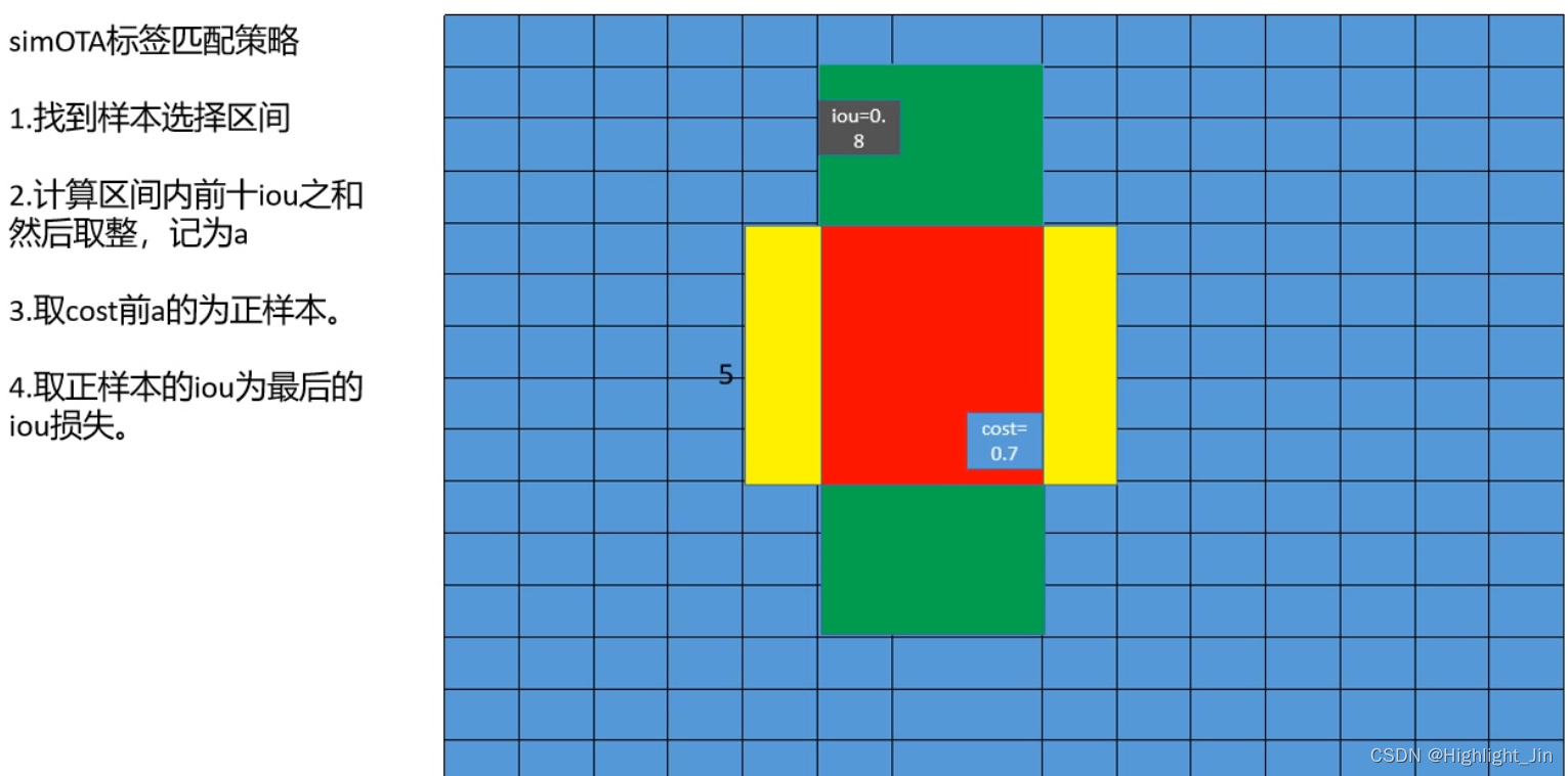
1.样本选择区间是43个格子。
2.每个格子与真实框的iou计算,计算出43个值,取前10个iou


 9044
9044


 被折叠的 条评论
为什么被折叠?
被折叠的 条评论
为什么被折叠?
 到【灌水乐园】发言


