「深度学习一遍过」必修21：基于Vgg16Net的MNIST手写数字识别

最新推荐文章于 2024-05-06 10:23:59 发布

荣仔！最靓的仔！

最新推荐文章于 2024-05-06 10:23:59 发布

阅读量3.5k

点赞数 8

分类专栏：「深度学习一遍过」必修篇文章标签：深度学习神经网络

本文链接：https://blog.csdn.net/IT_charge/article/details/120208229

版权

「深度学习一遍过」必修篇专栏收录该内容

28 篇文章 152 订阅

订阅专栏

本专栏用于记录关于深度学习的笔记，不光方便自己复习与查阅，同时也希望能给您解决一些关于深度学习的相关问题，并提供一些微不足道的人工神经网络模型设计思路。
专栏地址：「深度学习一遍过」必修篇

项目 GitHub 地址

项目心得

项目代码

项目 GitHub 地址

https://github.com/zhao302014/Classic_model_examples/tree/main/2014_Vgg16Net_MNISThttps://github.com/zhao302014/Classic_model_examples/tree/main/2014_Vgg16Net_MNIST

项目心得

2014 年——VGGNet：这是 2014 年牛津大学计算机视觉组和 Google DeepMind 公司研究员一起研发的深度网络模型。该网络结构被分为 11，13，16，19 层；该项目自己搭建了 VGGNet 网络并在 MNIST 手写数字识别项目中得到了应用。（注：该项目主要修改了 AlexNet 应用实例中的 net.py 代码，由于输入图片通道数依然为 3 通道，所以延续了 AlexNet 应用实例中的 train.py 与 test.py ，仅调小了其中的 banch_size （由 16 变为了 8），以避免因 CUDA 内存不足而引起的报错）

项目代码

vgg16

net.py

#!/usr/bin/python
# -*- coding:utf-8 -*-
# ------------------------------------------------- #
#      作者：赵泽荣
#      时间：2021年9月9日（农历八月初三）
#      个人站点：1.https://zhao302014.github.io/
#              2.https://blog.csdn.net/IT_charge/
#      个人GitHub地址：https://github.com/zhao302014
# ------------------------------------------------- #
import torch
from torch import nn
import torch.nn.functional as F

# --------------------------------------------------------------------------------- #
#  自己搭建一个 Vgg16 模型结构
#   · 提出时间：2014 年
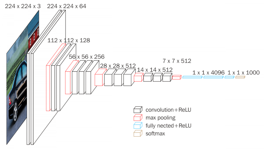
#   · VGGNet 的网络结构被分为 11，13，16，19 层，该实例实现 16 层的 VGGNet
#   · VGGNet 网络深，卷积层多
#   · 卷积核都是 3* 3 的或 1* 1 的，且同一层中 channel 的数量都是相同的。最大池化层全是 2*2。
#   · 每经过一个 pooling 层，channel 的数量会乘上2（即每次池化之后，Feature Map宽高降低一半，通道数量增加一倍）
#   · 意义：1.证明了更深的网络，能更好的提取特征；2.成为了后续很多网络的 backbone。
#   · 基准 Vgg16 截止到下述代码的 f16 层；由于本实例是手写数字识别（10分类问题），故再后续了一层全连接层 f_output
# --------------------------------------------------------------------------------- #
class MyVgg16Net(nn.Module):
    def __init__(self):
        super(MyVgg16Net, self).__init__()
        self.ReLU = nn.ReLU()   # 论文中的表格，每一大行对应是一个隐藏层,每个隐藏层计算完后的结果都需要经过 ReLU 激活函数进行激活
        # 第一段卷积神经网络：共 3 层，由 2 个卷积层和 1 个最大池化层构成
        self.c1 = nn.Conv2d(in_channels=3, out_channels=64, kernel_size=3, stride=1, padding=1)    # (224 - 3 + 2*1) / 1 + 1 = 224
        self.c2 = nn.Conv2d(in_channels=64, out_channels=64, kernel_size=3, stride=1, padding=1)   # (224 - 3 + 2*2) / 1 + 1 = 224
        self.s1 = nn.MaxPool2d(kernel_size=2, stride=2)
        # 第二段卷积神经网络：共 3 层，由 2 个卷积层和 1 个最大池化层构成
        self.c3 = nn.Conv2d(in_channels=64, out_channels=128, kernel_size=3, stride=1, padding=1)   # (112 - 3 + 2*1) / 1 + 1 = 112
        self.c4 = nn.Conv2d(in_channels=128, out_channels=128, kernel_size=3, stride=1, padding=1)  # (112 - 3 + 2*1) / 1 + 1 = 112
        self.s2 = nn.MaxPool2d(kernel_size=2, stride=2)
        # 第三段卷积神经网络：共 4 层，由 3 个卷积层和 1 个最大池化层构成
        self.c5 = nn.Conv2d(in_channels=128, out_channels=256, kernel_size=3, stride=1, padding=1)  # (56 - 3 + 2*1) / 1 + 1 = 56
        self.c6 = nn.Conv2d(in_channels=256, out_channels=256, kernel_size=3, stride=1, padding=1)  # (56 - 3 + 2*1) / 1 + 1 = 56
        self.c7 = nn.Conv2d(in_channels=256, out_channels=256, kernel_size=3, stride=1, padding=1)  # (56 - 3 + 2*1) / 1 + 1 = 56
        self.s3 = nn.MaxPool2d(kernel_size=2, stride=2)
        # 第四段卷积神经网络：共 4 层，由 3 个卷积层和 1 个最大池化层构成
        self.c8 = nn.Conv2d(in_channels=256, out_channels=512, kernel_size=3, stride=1, padding=1)  # (28 - 3 + 2*1) / 1 + 1 = 28
        self.c9 = nn.Conv2d(in_channels=512, out_channels=512, kernel_size=3, stride=1, padding=1)  # (28 - 3 + 2*1) / 1 + 1 = 28
        self.c10 = nn.Conv2d(in_channels=512, out_channels=512, kernel_size=3, stride=1, padding=1)  # (28 - 3 + 2*1) / 1 + 1 = 28
        self.s4 = nn.MaxPool2d(kernel_size=2, stride=2)
        # 第五段卷积神经网络：共 4 层，由 3 个卷积层和 1 个最大池化层构成
        self.c11 = nn.Conv2d(in_channels=512, out_channels=512, kernel_size=3, stride=1, padding=1)  # (28 - 3 + 2*1) / 1 + 1 = 28
        self.c12 = nn.Conv2d(in_channels=512, out_channels=512, kernel_size=3, stride=1, padding=1)  # (28 - 3 + 2*1) / 1 + 1 = 28
        self.c13 = nn.Conv2d(in_channels=512, out_channels=512, kernel_size=3, stride=1, padding=1)  # (28 - 3 + 2*1) / 1 + 1 = 28
        self.s5 = nn.MaxPool2d(kernel_size=2, stride=2)
        # 3 个全连接层置于 5 段卷积层之后
        self.flatten = nn.Flatten()
        self.f14 = nn.Linear(7*7*512, 4096)
        self.f15 = nn.Linear(4096, 4096)
        self.f16 = nn.Linear(4096, 1000)
        # 为满足该实例另加 ↓
        self.f_output = nn.Linear(1000, 10)

    def forward(self, x):                   # 输入shape: torch.Size([1, 3, 224, 224])
        x = self.c1(x)                      # shape: torch.Size([1, 64, 224, 224])
        x = self.c2(x)                      # shape: torch.Size([1, 64, 224, 224])
        x = self.s1(x)                      # shape: torch.Size([1, 64, 112, 112])
        x = self.ReLU(x)
        x = self.c3(x)                      # shape: torch.Size([1, 128, 112, 112])
        x = self.c4(x)                      # shape: torch.Size([1, 128, 112, 112])
        x = self.s2(x)                      # shape: torch.Size([1, 128, 56, 56])
        x = self.ReLU(x)
        x = self.c5(x)                      # shape: torch.Size([1, 256, 56, 56])
        x = self.c6(x)                      # shape: torch.Size([1, 256, 56, 56])
        x = self.c7(x)                      # shape: torch.Size([1, 256, 56, 56])
        x = self.s3(x)                      # shape: torch.Size([1, 256, 28, 28])
        x = self.ReLU(x)
        x = self.c8(x)                      # shape: torch.Size([1, 512, 28, 28])
        x = self.c9(x)                      # shape: torch.Size([1, 512, 28, 28])
        x = self.c10(x)                     # shape: torch.Size([1, 512, 28, 28])
        x = self.s4(x)                      # shape: torch.Size([1, 512, 14, 14])
        x = self.ReLU(x)
        x = self.c11(x)                     # shape: torch.Size([1, 512, 14, 14])
        x = self.c12(x)                     # shape: torch.Size([1, 512, 14, 14])
        x = self.c13(x)                     # shape: torch.Size([1, 512, 14, 14])
        x = self.s5(x)                      # shape: torch.Size([1, 512, 7, 7])
        x = self.ReLU(x)
        x = self.flatten(x)                 # shape: torch.Size([1, 25088])
        x = self.f14(x)                     # shape: torch.Size([1, 4096])
        x = self.f15(x)                     # shape: torch.Size([1, 4096])
        x = self.f16(x)                     # shape: torch.Size([1, 1000])
        # 为满足该实例另加 ↓
        x = self.f_output(x)                # shape: torch.Size([1, 10])
        # 全连接层之后使用了 softmax
        x = F.softmax(x, dim=1)             # shape: torch.Size([1, 10])
        return x


if __name__ == '__main__':
    x = torch.rand([1, 3, 224, 224])
    model = MyVgg16Net()
    y = model(x)
    
# ---------------------------------------------------------------------------------------------------------------------------------------------------------- #
#  已知：在 VGG16 中，使用 2 个 3*3 卷积核来代替 5*5 卷积核；这样做的主要目的是在保证具有相同感受野的条件下，提升了网络的深度，在一定程度上提升了神经网络的效果。
#  问：为什么 1 个 5*5 的卷积核可以由 2 个 3*3 的卷积核替代？
#  答：我们假设图片是 28*28 的
#      我们使用 5*5 的卷积核对其卷积，步长为 1，得到的结果是：(28-5)/1+1=24
#      然后我们使用 2 个卷积核为 3*3 的，这里的 2 个是指 2 层：
#                                   第一层 3*3：得到的结果是：(28-3)/1+1=26
#                                   第二层 3*3：得到的结果是：(26-3)/1+1=24
#      所以我们的最终结果和 5*5 的卷积核是一样的！！！
# ---------------------------------------------------------------------------------------------------------------------------------------------------------- #

train.py

#!/usr/bin/python
# -*- coding:utf-8 -*-
# ------------------------------------------------- #
#      作者：赵泽荣
#      时间：2021年9月9日（农历八月初三）
#      个人站点：1.https://zhao302014.github.io/
#              2.https://blog.csdn.net/IT_charge/
#      个人GitHub地址：https://github.com/zhao302014
# ------------------------------------------------- #
import torch
from torch import nn
from net import MyVgg16Net
import numpy as np
from torch.optim import lr_scheduler
from torchvision import datasets, transforms

data_transform = transforms.Compose([
    transforms.Scale(224),    # 缩放图像大小为 224*224
    transforms.ToTensor()     # 仅对数据做转换为 tensor 格式操作
])

# 加载训练数据集
train_dataset = datasets.MNIST(root='./data', train=True, transform=data_transform, download=True)
# 给训练集创建一个数据集加载器
train_dataloader = torch.utils.data.DataLoader(dataset=train_dataset, batch_size=8, shuffle=True)
# 加载测试数据集
test_dataset = datasets.MNIST(root='./data', train=False, transform=data_transform, download=True)
# 给测试集创建一个数据集加载器
test_dataloader = torch.utils.data.DataLoader(dataset=train_dataset, batch_size=8, shuffle=True)

# 如果显卡可用，则用显卡进行训练
device = "cuda" if torch.cuda.is_available() else 'cpu'

# 调用 net 里定义的模型，如果 GPU 可用则将模型转到 GPU
model = MyVgg16Net().to(device)

# 定义损失函数（交叉熵损失）
loss_fn = nn.CrossEntropyLoss()
# 定义优化器（SGD：随机梯度下降）
optimizer = torch.optim.SGD(model.parameters(), lr=1e-3, momentum=0.9)
# 学习率每隔 10 个 epoch 变为原来的 0.1
lr_scheduler = lr_scheduler.StepLR(optimizer, step_size=10, gamma=0.1)

# 定义训练函数
def train(dataloader, model, loss_fn, optimizer):
    loss, current, n = 0.0, 0.0, 0
    for batch, (X, y) in enumerate(dataloader):
        # 单通道转为三通道
        X = np.array(X)
        X = X.transpose((1, 0, 2, 3))             # array 转置
        image = np.concatenate((X, X, X), axis=0)
        image = image.transpose((1, 0, 2, 3))     # array 转置回来
        image = torch.tensor(image)               # 将 numpy 数据格式转为 tensor
        # 前向传播
        image, y = image.to(device), y.to(device)
        output = model(image)
        cur_loss = loss_fn(output, y)
        _, pred = torch.max(output, axis=1)
        cur_acc = torch.sum(y == pred) / output.shape[0]
        # 反向传播
        optimizer.zero_grad()
        cur_loss.backward()
        optimizer.step()
        loss += cur_loss.item()
        current += cur_acc.item()
        n = n + 1
    print('train_loss：' + str(loss / n))
    print('train_acc：' + str(current / n))

# 定义测试函数
def test(dataloader, model, loss_fn):
    # 将模型转换为验证模式
    model.eval()
    loss, current, n = 0.0, 0.0, 0
    # 非训练，推理期用到（测试时模型参数不用更新，所以 no_grad）
    with torch.no_grad():
        for batch, (X, y) in enumerate(dataloader):
            # 单通道转为三通道
            X = np.array(X)
            X = X.transpose((1, 0, 2, 3))  # array 转置
            image = np.concatenate((X, X, X), axis=0)
            image = image.transpose((1, 0, 2, 3))  # array 转置回来
            image = torch.tensor(image)  # 将 numpy 数据格式转为 tensor
            image, y = image.to(device), y.to(device)
            output = model(image)
            cur_loss = loss_fn(output, y)
            _, pred = torch.max(output, axis=1)
            cur_acc = torch.sum(y == pred) / output.shape[0]
            loss += cur_loss.item()
            current += cur_acc.item()
            n = n + 1
        print('test_loss：' + str(loss / n))
        print('test_acc：' + str(current / n))

# 开始训练
epoch = 100
for t in range(epoch):
    lr_scheduler.step()
    print(f"Epoch {t + 1}\n----------------------")
    train(train_dataloader, model, loss_fn, optimizer)
    test(test_dataloader, model, loss_fn)
    torch.save(model.state_dict(), "save_model/{}model.pth".format(t))    # 模型保存
print("Done!")

test.py

#!/usr/bin/python
# -*- coding:utf-8 -*-
# ------------------------------------------------- #
#      作者：赵泽荣
#      时间：2021年9月9日（农历八月初三）
#      个人站点：1.https://zhao302014.github.io/
#              2.https://blog.csdn.net/IT_charge/
#      个人GitHub地址：https://github.com/zhao302014
# ------------------------------------------------- #
import torch
from net import MyVgg16Net
import numpy as np
from torch.autograd import Variable
from torchvision import datasets, transforms
from torchvision.transforms import ToPILImage

data_transform = transforms.Compose([
    transforms.Scale(224),     # 缩放图像大小为 224*224
    transforms.ToTensor()      # 仅对数据做转换为 tensor 格式操作
])

# 加载训练数据集
train_dataset = datasets.MNIST(root='./data', train=True, transform=data_transform, download=True)
# 给训练集创建一个数据集加载器
train_dataloader = torch.utils.data.DataLoader(dataset=train_dataset, batch_size=8, shuffle=True)
# 加载测试数据集
test_dataset = datasets.MNIST(root='./data', train=False, transform=data_transform, download=True)
# 给测试集创建一个数据集加载器
test_dataloader = torch.utils.data.DataLoader(dataset=train_dataset, batch_size=8, shuffle=True)

# 如果显卡可用，则用显卡进行训练
device = "cuda" if torch.cuda.is_available() else 'cpu'

# 调用 net 里定义的模型，如果 GPU 可用则将模型转到 GPU
model = MyVgg16Net().to(device)
# 加载 train.py 里训练好的模型
model.load_state_dict(torch.load("./save_model/99model.pth"))

# 获取预测结果
classes = [
    "0",
    "1",
    "2",
    "3",
    "4",
    "5",
    "6",
    "7",
    "8",
    "9",
]

# 把 tensor 转成 Image，方便可视化
show = ToPILImage()
# 进入验证阶段
model.eval()
# 对 test_dataset 里 10000 张手写数字图片进行推理
for i in range(len(test_dataset)):
    x, y = test_dataset[i][0], test_dataset[i][1]
    # tensor格式数据可视化
    show(x).show()
    # 扩展张量维度为 4 维
    x = Variable(torch.unsqueeze(x, dim=0).float(), requires_grad=False).to(device)
    # 单通道转为三通道
    x = x.cpu()
    x = np.array(x)
    x = x.transpose((1, 0, 2, 3))          # array 转置
    x = np.concatenate((x, x, x), axis=0)
    x = x.transpose((1, 0, 2, 3))      # array 转置回来
    x = torch.tensor(x).to(device)   # 将 numpy 数据格式转为 tensor，并转回 cuda 格式
    with torch.no_grad():
        pred = model(x)
        # 得到预测类别中最高的那一类，再把最高的这一类对应classes中的哪一个标签
        predicted, actual = classes[torch.argmax(pred[0])], classes[y]
        # 最终输出预测值与真实值
        print(f'Predicted: "{predicted}", Actual: "{actual}"')
© 2021 GitHub, Inc.

欢迎大家交流评论，一起学习

希望本文能帮助您解决您在这方面遇到的问题

感谢阅读
END

荣仔！最靓的仔！

关注

8
点赞
踩
47

收藏

觉得还不错? 一键收藏
打赏
5
评论
「深度学习一遍过」必修21：基于Vgg16Net的MNIST手写数字识别

本专栏用于记录关于深度学习的笔记，不光方便自己复习与查阅，同时也希望能给您解决一些关于深度学习的相关问题，并提供一些微不足道的人工神经网络模型设计思路。专栏地址：「深度学习一遍过」必修篇目录项目 GitHub 地址项目心得项目代码项目 GitHub 地址https://github.com/zhao302014/Classic_model_examples/tree/main/2014_Vgg16Net_MNISThttps://github.com/zhao30...
复制链接

扫一扫

专栏目录

「深度学习一遍过」必修21：基于Vgg16Net的MNIST手写数字识别

项目 GitHub 地址

项目心得

项目代码

欢迎大家交流评论，一起学习 希望本文能帮助您解决您在这方面遇到的问题 感谢阅读 END

“相关推荐”对你有帮助么？

欢迎大家交流评论，一起学习

希望本文能帮助您解决您在这方面遇到的问题

感谢阅读
END