XGBoost math Derivation 通俗易懂的详细推导

往期文章链接目录

Bagging v.s. Boosting:

Bagging:
Leverages unstable base learners that are weak because of overfitting.

Boosting:
Leverages stable base learners that are weak because of underfitting.

XGBoost

Learning Process through XGBoost:

1. How to set a objective function.
2. Hard to solve directly, how to approximate.
3. How to add tree structures into the objective function.
4. Still hard to optimize, then have to use greedy algorithms.

Step 1. How to set an objective function

Suppose we trained $K$ trees, then the prediction for the ith sample is
$${\hat{y}}_i=\sum _{k=1}^K{f}_k(x_i),f_k\in \mathcal{F}$$
where $K$ is the number of trees, $f$ is a function in the functional space $\mathcal{F}$, and $\mathcal{F}$ is the set of all possible CARTs.

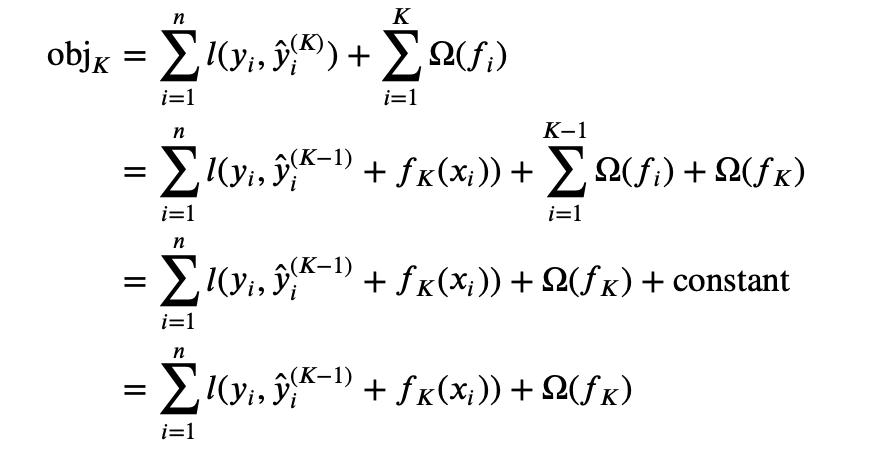
The objective function to be optimized is given by
$$\text{obj}=\sum _i^{n}l(y_i,{\hat{y}}_i)+\sum _{k=1}^K\Omega (f_k)$$
The first term is the loss function and the second term controls trees’ complexity. We see the undefined terms in this objective function are the loss function $l$ and model complexity $\Omega (f_i)$. Functions $f_i$ are what we need to learn, each containing the structure of the tree and the leaf scores.

we use an additive strategy to build the model. That is, fix what we have learned, and add one new tree at a time. This is called Additive Training.

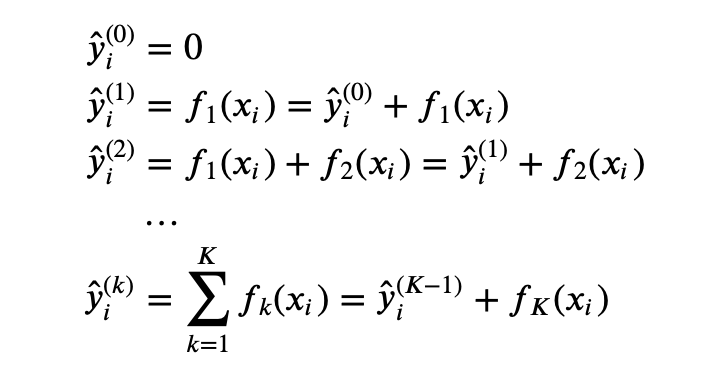
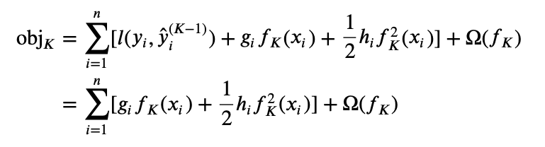
Note that given $x_i$, the prediction ${\hat{y}}_i^{(K)}={\hat{y}}_i^{(K-1)}+f_K(x_i)$, where the term ${\hat{y}}_i^{(K-1)}$ is known and only $f_K(x_i)$ is unknown.

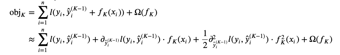
Now, we can rewrite the objective function as

Step 2. Hard to solve directly, how to approximate

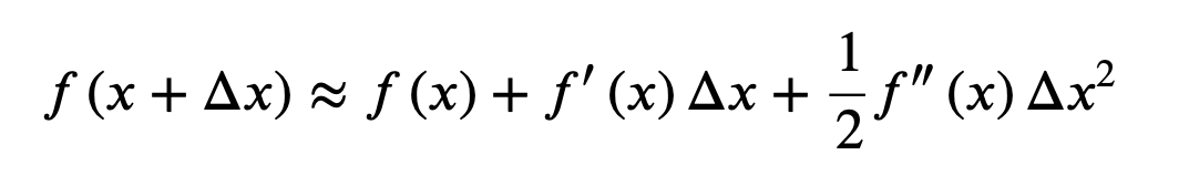
If the loss function is the MSE, then the objective function has a nice form. But for a general loss function, it is hard to optimize directly. Therefore, we need to approximate it. Here, we use second order Taylor approximation

So we can re-write the objective function as

If we define constant term $g_i$, $h_i$ as
$$\begin{gathered} g_i={\partial }_{{\hat{y}}_i^{(K-1)}}l(y_i,{\hat{y}}_i^{(K-1)}) \\ {f}_i={\partial }_{{\hat{y}}_i^{(K-1)}}^{2}l(y_i,{\hat{y}}_i^{(K-1)}) \end{gathered}$$
Also, since previous $K-1$ trees are fixed, we have ${\sum }_{i=1}^{n}l(y_i,{\hat{y}}_i^{(K-1)})$ fixed. Then we can write the objective function as

Now, all previous trees’ information is stored in terms $g_i$ and $h_i$. That’s how the $K$th tree is related to previous trees. Our new objective function now is
$${\text{obj}}_K=\sum _{i=1}^n[g_i{f}_K(x_i)+\frac{1}{2}{h}_i{f}_K^2(x_i)]+\Omega (f_K)$$
The unknown at this point are $f_K$ and $\Omega (f_K)$.

Step 3. How to add tree structures into the objective function

Redefine a tree:

• Define I j = { i ∣ q ( x i ) = j } I_j = \{i|q(x_i)=j\} Ij​={i∣q(xi​)=j} to be the set of indices of data points assigned to the 𝑗-th leaf.
• $T$ is the number of leaves.
• $q(x_i)$ is which leaf the $i$-th sample is assigned to. Term $q(x)$ defines the tree structure.
• $w_{q(x_i)}$ is the score of the assigned leaf.
• In XGBoost, we define the complexity as $\Omega (f)=\gamma T+\frac{1}{2}\lambda {\sum }_{j=1}^T{w}_j^2$

Now the revised objective function is

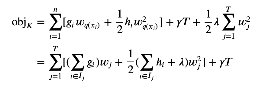
Define $G_j={\sum }_{i\in I_j}{g}_i$ and $H_j={\sum }_{i\in I_j}{h}_i$ constants. The the objective function is
$${\text{obj}}_K=\sum _{j=1}^T[G_j{w}_j+\frac{1}{2}(H_j+\lambda )w_j^2]+\gamma T$$

Right now, the only unknown is $w_j$, which is independent respect to other terms. Take the derivative and set it to zero, we have
$$w_j=-\frac{G_j}{H_j+\lambda }$$
Then the objective function achieve its minimum at
$${\text{obj}}_K=-\frac{1}{2}\sum _{j=1}^T\frac{G_j^2}{H_j+\lambda }+\gamma T$$

Step 4. Still hard to optimize, then have to use greedy algorithms

For any tree structure, we are now able to find the minimum value of the objective function. Ideally we would brute force all possible tree structures and pick the one with the minimum objective function. However, this is impossible in practice and we use greedy algorithm instead. When we build decision trees, we use entropy to calculate the information gain. Now we are still going to use information gain, but the formula changes to

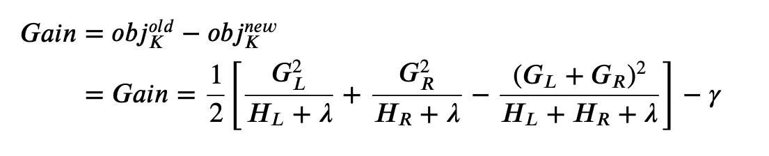
where $L$ is the left leaf and $R$ is the right leaf.

---

Reference:
https://xgboost.readthedocs.io/en/latest/tutorials/model.html

往期文章链接目录