


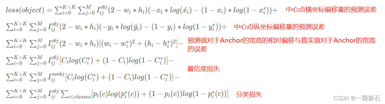
YOLO v3的损失函数构成及表达式
YOLO v3的损失函数由定位损失、置信度损失以及分类损失三部分组成。相信下边的公式大家看过很多遍了,我标明了各个损失对应的部分。
题外话
在网上查阅了很多资料,很多人都反应说复现的代码和DarkNet开源代码在LOSS的设计上是有出入的。比如原来的BCE损失改成了MSE损失(这个问题在一些大佬们经过梯度反向推导之后发现这两种损失的梯度是一样的,所以两种都可以)。对于损失其它的改变我们也可以理解,毕竟研究的是一门炼丹玄学,每个人碰到的业务场景和环境也不一样,选择不同的方式也可以接受,大家的目的都是跑出最好的结果。
在分析YOLO v3的LOSS之前,有必要先了解以下BCE(Binary CrossEntropy)。因为在YOLO v3里,很多部分的损失都是用BCE计算的。比如类别分类损失,每张图片里不只有一个类别的目标(比如人和鸟可能同时出现),是一个多标签分类问题,而不是简单的二分类问题,所以在YOLO v3里作者把激活函数从Softmax换成了Sigmoid(Softmax会扩大最大输出值对应类别的概率值,从而抑制其他类别,不利于多标签分类),部分损失改由BCE计算。详情请移步参考: BCE损失函数.
YOLO v3的模型输出与多尺度预测
YOLO v3为了完成多尺度的目标检测,使用了FPN的结构,最终输出三种不同尺度的特征图(13×13、26×26、39×39)分别预测不同大小的目标。每种尺寸的特征图都要输出自己负责目标的预测信息(中心点偏移、宽高偏移、置信度、类别)。因此三种不同的特征图的预测结果都要计算与target的损失,并且相加进行反向梯度传播优化。
研究LOSS的思维
按照深度学习的架构,为了计算LOSS,我们需要先获取到目标值(Target)和预测值(Prediction)。
YOLO v3是一个经典的目标检测框架,目标检测的目的是要定位出图像中目标的位置,并且判断该目标的类别。因此它的模型预测输出为预测框的位置信息以及框内物体的类别。除此之外,YOLO v3还预测输出了当前特征点中是否包含物体的置信度。
获取目标真实值target
我们先去源码里的Dataloader里去看一看网络使用的target是什么以及格式是什么样的。
class YoloDataset(Dataset):
    def __init__(self, annotation_lines, input_shape, num_classes):
        super(YoloDataset, self).__init__()
        self.annotation_lines   = annotation_lines  # 原始的标注信息[图片地址、真实框信息(左上角和右下角坐标)]
        self.input_shape        = input_shape  # 模型输入的尺寸
        self.num_classes        = num_classes  # 数据集中目标的类别数
        self.length             = len(self.annotation_lines)  # 真实框的数量

    def __len__(self):
        return self.length  # 获取数据集的体量

    def __getitem__(self, index):  # 获取一个数据样本
        index       = index % self.length  # 当前用于获取数据样本的索引
        image, box  = self.get_random_data(self.annotation_lines[index], self.input_shape[0:2])
        image       = np.transpose(preprocess_input(np.array(image, dtype=np.float32)), (2, 0, 1))
        box         = np.array(box, dtype=np.float32)
        if len(box) != 0:
            box[:, [0, 2]] = box[:, [0, 2]] / self.input_shape[1]
            box[:, [1, 3]] = box[:, [1, 3]] / self.input_shape[0]

            box[:, 2:4] = box[:, 2:4] - box[:, 0:2]
            box[:, 0:2] = box[:, 0:2] + box[:, 2:4] / 2
        return image, box

    def get_random_data(self, annotation_line, input_shape):
        line    = annotation_line.split()
        #------------------------------#
        #   读取图像并转换成RGB图像
        #------------------------------#
        image   = Image.open(line[0])
        image   = cvtColor(image)
        #------------------------------#
        #   获得图像的高宽与目标高宽
        #------------------------------#
        iw, ih  = image.size
        h, w    = input_shape
        #------------------------------#
        #   获得预测框
        #------------------------------#
        box     = np.array([np.array(list(map(int,box.split(',')))) for box in line[1:]])

        if not random:
            scale = min(w/iw, h/ih)  # 计算图像缩放的尺度
            nw = int(iw*scale)  # 缩放后的宽
            nh = int(ih*scale)  # 缩放后的高
            dx = (w-nw)//2  # 缩放后的图像转换为模型输入尺寸在宽的维度上需要扩展的灰色像素尺寸
            dy = (h-nh)//2  # 缩放后的图像转换为模型输入尺寸在高的维度上需要扩展的灰色像素尺寸

            #---------------------------------#
            #   将图像多余的部分加上灰条
            #---------------------------------#
            image       = image.resize((nw,nh), Image.BICUBIC)  # 采用双线性插值对图像进行resize到[nw, nh]
            new_image   = Image.new('RGB', (w,h), (128,128,128))  # 创建一张尺寸为模型输入大小的灰色图像
            new_image.paste(image, (dx, dy))  # resize好的图像粘贴到新创建的图像上
            image_data  = np.array(new_image, np.float32)

            # ---------------------------------#
            #   对真实框进行调整
            # ---------------------------------#
            if len(box)>0:
                np.random.shuffle(box)  # 真实框打乱顺序,有利于训练
                box[:, [0,2]] = box[:, [0,2]] * nw/iw + dx  # 计算原始图像上的真实框x轴坐标转换到新图像上的坐标
                box[:, [1,3]] = box[:, [1,3]] * nh/ih + dy  # 计算原始图像上的真实框y轴坐标转换到新图像上的坐标
                box[:, 0:2][box[:, 0:2] < 0] = 0  # 转换后的坐标超出图像范围,限制在图像的边界处
                box[:, 2][box[:, 2] > w] = w
                box[:, 3][box[:, 3] > h] = h
                box_w = box[:, 2] - box[:, 0]  # 这说明原始GT框的形式为[x1,y1,x2,y2]
                box_h = box[:, 3] - box[:, 1]   # 计算转换后的真实框的宽高信息
                box = box[np.logical_and(box_w > 1, box_h > 1)] # 只保留图像内的真实框

            return image_data, box  # 此处返回的box中位置信息依旧是左上角和右下角的坐标

只看代码可能还是比较迷糊,结合上图观察,经过DATaloader输出的target位置信息是模型输入图像上左上角和右上角的x, y坐标。通过读论文我们知道,在位置信息上YOLO v3预测的是与负责该目标的anchor中心点的偏移量,所以我们还要根据target中的左上角和右上角坐标计算出target的中心点与宽高,并计算target中心点和宽高与anchor之间的偏移量。这样以anchor为参考系,计算prediction和target之间的差距。

预测值的获取
prediction = input.view(bs, len(self.anchors_mask[l]), self.bbox_attrs, in_h, in_w).permute(0, 1, 3, 4, 2).contiguous()
其中:
bs:Batch_size的大小
len(self.anchors_mask[l]:负责当前尺寸的特征层的anchor数目(YOLO v3中每种尺寸下的特征层分配3种尺寸的anchor)
self.bbox_attrs:预测框的属性集合[ t x t_x tx, t y t_y ty, t w t_w tw, t h t_h th, c l a s s class class]
in_h, in_w:当前特征图的高和宽
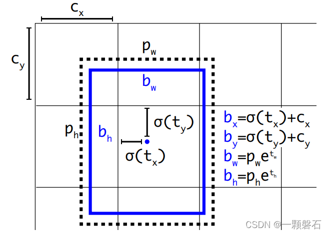
读原论文的时候可以发现,模型预测的输出是预测框相对于anchor的偏移量
t
x
t_x
tx,
t
y
t_y
ty,
t
w
t_w
tw,
t
h
t_h
th,通过上边图里的公式我们可以根据预测的偏移量计算出预测框的中心点位置以及宽高。
我们上边获取的target里边包含的其实是
b
x
,
b
y
,
b
w
,
b
h
b_x, b_y, b_w, b_h
bx,by,bw,bh的真实值,记作
b
x
∗
,
b
y
∗
,
b
w
∗
,
b
h
∗
{b_x}^*, {b_y}^*, {b_w}^*, {b_h}^*
bx∗,by∗,bw∗,bh∗。
因为图中的
b
x
和
t
x
b_x和t_x
bx和tx的对应关系,我们需要对获取到的target做一个如下的变换:
σ ( t x ∗ ) = b x ∗ − c x σ({t_x}^*)={b_x}^*-c_x σ(tx∗)=bx∗−cx
σ ( t y ∗ ) = b y ∗ − c y σ({t_y}^*)={b_y}^*-c_y σ(ty∗)=by∗−cy
t x ∗ = l o g ( b w ∗ / p w ) {t_x}^*=log({b_w}^*/p_w) tx∗=log(bw∗/pw)
t h ∗ = l o g ( b h ∗ / p h ) {t_h}^*=log({b_h}^*/p_h) th∗=log(bh∗/ph)
接下来,我们就要通过[ t x t_x tx, t y t_y ty, t w t_w tw, t h t_h th]和[ t x ∗ , t y ∗ , t w ∗ , t h ∗ {t_x}^*, {t_y}^*, {t_w}^*, {t_h}^* tx∗,ty∗,tw∗,th∗,]计算定位损失了。定位损失就是使用的BCE损失计算的
这里要说的一点是,只有当前特征图的点负责预测一个目标物体的时候,我们才会计算它的定位损失、分类损失,只有置信度损失是所有特征点参与计算的。
就如同文章开头公式里写的那样, I i j o b j {I_{ij}}^{obj} Iijobj如果等于1,代表的是第i个特征点的第j个anchor有一个负责预测的目标;如果等于0,代表第i个特征点的第j个anchor没有要负责预测的目标。 I i j n o o b j {I_{ij}}^{noobj} Iijnoobj代表的是相反的含义。
# -----------------------------------------------------------#
#    使用BCE计算中心点偏移值的loss
# -----------------------------------------------------------#
loss_x = torch.mean(self.BCELoss(x[obj_mask], y_true[..., 0][obj_mask]) * box_loss_scale)
loss_y = torch.mean(self.BCELoss(y[obj_mask], y_true[..., 1][obj_mask]) * box_loss_scale)
# -----------------------------------------------------------#
#    用MSE计算宽高调整值的loss
# -----------------------------------------------------------#
loss_w = torch.mean(self.MSELoss(w[obj_mask], y_true[..., 2][obj_mask]) * box_loss_scale)
loss_h = torch.mean(self.MSELoss(h[obj_mask], y_true[..., 3][obj_mask]) * box_loss_scale)
#   中心点偏移值 + 宽高偏移值 = 总体的定位损失值
loss_loc = (loss_x + loss_y + loss_h + loss_w) * 0.1
#   使用BCE计算分类(多标签分类)的loss
loss_cls = torch.mean(self.BCELoss(pred_cls[obj_mask], y_true[..., 5:][obj_mask]))
#   对定位损失和分类损失做权重分配,使网络的综合性能更强
loss += loss_loc * self.box_ratio + loss_cls * self.cls_ratio
#   使用BCE计算置信度损失
loss_conf   = torch.mean(self.BCELoss(conf, obj_mask.type_as(conf))[noobj_mask.bool() | obj_mask])  # *********
loss        += loss_conf * self.balance[l] * self.obj_ratio
从代码中我们看到了,obj_mask就是上边公式里的 I i j o b j {I_{ij}}^{obj} Iijobj,在计算的loss_x, loss_y, loss_w, loss_h, loss_cls的时候只考虑了 I i j o b j {I_{ij}}^{obj} Iijobj=1的预测框;而在计算置信度损失的时候 I i j o b j {I_{ij}}^{obj} Iijobj=1和 I i j n o o b j {I_{ij}}^{noobj} Iijnoobj=1的预测框都参与了计算。还有一个参数是box_loss_scale,该参数是为了兼顾小目标检测的性能,目标的尺寸越小,box_loss_scale越大,从而损失越大。
总结
YOLO v3是一种单阶段带anchor设计的目标检测框架,并且通过引入FPN完成多尺度目标的检测。损失包含定位损失,置信度损失,分类损失三部分,有MSE和BCE两种LOSS计算得到。模型的检测头预测输出的定位信息为预测框相对于预设anchor的偏移量( t x t_x tx, t y t_y ty, t w t_w tw, t h t_h th),再通过真实目标信息target和anchor之间的偏移量计算LOSS。此篇博客是自己学习过程中的记录,仅限于于个人理解,有不正确的地方希望大家能够指出,虚心学习一起交流。希望能帮助到朋友们!


 962
962


 被折叠的 条评论
为什么被折叠?
被折叠的 条评论
为什么被折叠?
 到【灌水乐园】发言


