


一、实验要求
1.使用卷积神经网络实现图片分类,数据集为OxFlowers17;
二、实验环境
Anaconda2-4.3.1(Python2.7),tensorflow-cpu。
三、实验原理
3.1 数据读取
已知数据集是连续80个样本为一个分类,有17个类别,所以一共只有1360个样本,所以首先用一个函数把每一类的样本分到一个文件夹,文件夹的名字从0开始命名,接着进行数据的读取,由于本次实验使用的数据集比较小,因而没有划分出验证集,根据官网给出的划分数据集的方法,把验证集也划分给训练集,以丰富训练集,最后得到1020个训练样本和340个测试样本。
对应代码:loadData.py
# -*- coding: UTF-8 -*-

import os
import numpy as np
import scipy.io as sio
from PIL import Image

dir='../oxflower17/jpg/'

def to_categorical(y, nb_classes):
    y = np.asarray(y, dtype='int32')
    if not nb_classes:
        nb_classes = np.max(y)+1
    Y = np.zeros((1, nb_classes))
    Y[0,y] = 1.
    return Y

def build_class_directories(dir):
    dir_id = 0
    class_dir = os.path.join(dir, str(dir_id))
    if not os.path.exists(class_dir):
        os.mkdir(class_dir)
    for i in range(1, 1361):
        fname = "image_" + ("%.4i" % i) + ".jpg"
        os.rename(os.path.join(dir, fname), os.path.join(class_dir, fname))
        if i % 80 == 0 and dir_id < 16:
            dir_id += 1
            class_dir = os.path.join(dir, str(dir_id))
            os.mkdir(class_dir)

def get_input(resize=[224,224]):
    print 'Load data...'

    getJPG = lambda filePath: np.array(Image.open(filePath).resize(resize))

    dataSet=[];labels=[];choose=1
    classes = os.listdir(dir)
    for index, name in enumerate(classes):
        class_path = dir+ name + "/"
        if os.path.isdir(class_path):
            for img_name in os.listdir(class_path):
                img_path = class_path + img_name
                img_raw = getJPG(img_path)
                dataSet.append(img_raw)
                y=to_categorical(int(name),17)
                labels.append(y)

    datasplits = sio.loadmat('../oxflower17/datasplits.mat')
    keys = [x + str(choose) for x in ['val', 'trn', 'tst']]
    train_set, vall_set, test_set = [set(list(datasplits[name][0])) for name in keys]
    train_data, train_label,test_data ,test_label= [],[],[],[]

    for i in range(len(labels)):
        num = i + 1
        if num in test_set:
            test_data.append(dataSet[i])
            test_label.extend(labels[i])
        else:
            train_data.append(dataSet[i])
            train_label.extend(labels[i])
    train_data = np.array(train_data, dtype='float32')
    train_label = np.array(train_label, dtype='float32')
    test_data = np.array(test_data, dtype='float32')
    test_label = np.array(test_label, dtype='float32')
    return train_data, train_label,test_data ,test_label

def batch_iter(data, batch_size, num_epochs, shuffle=True):
    data = np.array(data)
    data_size = len(data)
    num_batches_per_epoch = int((len(data)-1)/batch_size) + 1
    for epoch in range(num_epochs):
        # Shuffle the data at each epoch
        if shuffle:
            shuffle_indices = np.random.permutation(np.arange(data_size))
            shuffled_data = data[shuffle_indices]
        else:
            shuffled_data = data
        for batch_num in range(num_batches_per_epoch):
            start_index = batch_num * batch_size
            end_index = min((batch_num + 1) * batch_size, data_size)
            yield shuffled_data[start_index:end_index]

if __name__=='__main__':
    #build_class_directories(os.path.join(dir))
    train_data, train_label,test_data, test_label=get_input()
    print len(train_data),len(test_data)
3.2 模型介绍
本次实验使用的是AlexNet模型,AlexNet共有八层,其前五层是卷积层,后三层是全连接层。最后一个全连接层的输出具有17个输出单元。
其中第一个卷积层conv1,采用了96个11 * 11 的kernel,stride为4,第二层卷积层conv2采用了192个5 * 5 的kernel,stride为1,后面三层的分别为384个3*3的kernel,256个3*3的kernel,256个3*3的kernel,所有的stride均为1,并且只有第一,第二和第五层有pooling层和Norm(norm1)变换。为了防止过拟合,在这三层设置了dropout,dropout值为0.5,最后是三层的全连接层,输出为17个神经单元,所有的激活函数都是relu函数,我们把这些东西全部放在一个类里进行实现。具体可见代码及下图1用tensorboard生成模型图。
分类问题的标准损失函数是交叉熵损失函数加上最后一层全连接层参数正则化*0.01。
对应代码:AlexNet.py
# -*- coding: utf-8 -*-

import tensorflow as tf
import numpy as np


def conv(input,fh,fw,n_out,name):
    n_in = input.get_shape()[-1].value
    with tf.name_scope(name) as scope:
        filter = tf.get_variable(scope+"w", shape=[fh, fw, n_in, n_out], dtype=tf.float32,
                                 initializer=tf.contrib.layers.xavier_initializer_conv2d())
        conv = tf.nn.conv2d(input, filter, [1,4,4,1], padding='SAME')
        bias_val = tf.constant(0.0, shape=[n_out], dtype=tf.float32)
        biases = tf.Variable(bias_val, trainable=True, name='b')
        z = tf.nn.bias_add(conv, biases)
        relu = tf.nn.relu(z, name=scope)
        return relu

def conv_layer(input,fh,fw,n_out,name):
    n_in = input.get_shape()[-1].value
    with tf.name_scope(name) as scope:
        filter = tf.get_variable(scope+"w", shape=[fh, fw, n_in, n_out], dtype=tf.float32,
                                 initializer=tf.contrib.layers.xavier_initializer_conv2d())
        conv = tf.nn.conv2d(input, filter, [1,1,1,1], padding='SAME')
        bias_val = tf.constant(0.0, shape=[n_out], dtype=tf.float32)
        biases = tf.Variable(bias_val, trainable=True, name='b')
        z = tf.nn.bias_add(conv, biases)
        relu = tf.nn.relu(z, name=scope)
        return relu

def full_connected_layer(input, n_out,name):
    shape = input.get_shape().as_list()
    dim = 1
    for d in shape[1:]:
        dim *= d
    x = tf.reshape(input, [-1, dim])
    n_in = x.get_shape()[-1].value
    with tf.name_scope(name) as scope:
        filter = tf.get_variable(scope+"w", shape=[n_in, n_out], dtype=tf.float32,
                                 initializer=tf.contrib.layers.xavier_initializer_conv2d())
        bias_val = tf.constant(0.1, shape=[n_out], dtype=tf.float32)
        biases = tf.Variable(bias_val, name='b')
        fc = tf.nn.relu_layer(input, filter, biases, name=scope)
        return fc

def max_pool_layer(input,name):
    return tf.nn.max_pool(input, ksize=[1,3,3,1], strides=[1,2,2,1],padding='SAME', name=name)

def norm(name, l_input, lsize=4):
    return tf.nn.lrn(l_input, lsize, bias=1.0, alpha=0.001 / 9.0, beta=0.75, name=name)

class CNN(object):
    def __init__(
      self, num_classes,l2_reg_lambda=0.01):

        self.input_x = tf.placeholder(tf.float32, [None, 224,224,3], name="input_x")
        self.input_y = tf.placeholder(tf.float32, [None, num_classes], name="input_y")
        self.dropout_keep_prob = tf.placeholder(tf.float32, name="dropout_keep_prob")
        l2_loss = tf.constant(0.1)

        with tf.name_scope("conv-maxpool"):
            # first layer
            self.conv1_1 = conv(self.input_x,fh=11, fw=11,n_out=96,name="conv1_1")
            self.pool1 = max_pool_layer(self.conv1_1,name='pool1')
            self.norm1 = norm('norm1', self.pool1, lsize=4)
            self.norm1 = tf.nn.dropout(self.norm1, self.dropout_keep_prob)

            # second layer
            self.conv2_1 = conv_layer(self.norm1, fh=5, fw=5, n_out=192,name='conv2_1')
            self.pool2 = max_pool_layer(self.conv2_1, name='pool2')
            self.norm2 = norm('norm2', self.pool2, lsize=4)
            self.norm2 = tf.nn.dropout(self.norm2, self.dropout_keep_prob)

            # Third layer
            self.conv3_1 = conv_layer(self.norm2, fh=3, fw=3, n_out=384, name='conv3_1')
            self.conv3_2 = conv_layer(self.conv3_1,fh=3, fw=3, n_out=256, name='conv3_2')
            self.conv3_3 = conv_layer(self.conv3_2, fh=3, fw=3, n_out=256, name='conv3_3')
            self.pool3 = max_pool_layer(self.conv3_3, name='pool3')
            self.norm3 = norm('self.norm3', self.pool3, lsize=4)
            self.norm3 = tf.nn.dropout(self.norm3,self.dropout_keep_prob)


        # Combine all the pooled features
        shape = self.norm3.get_shape().as_list()
        self.dim = 1
        for d in shape[1:]:
            self.dim *= d
        self.h_pool_flat= tf.reshape(self.norm3, [-1, self.dim])

        with tf.name_scope("output"):
            W1 = tf.get_variable(
                "W1",
                shape=[self.dim, 4096],
                initializer=tf.contrib.layers.xavier_initializer())
            b1 = tf.Variable(tf.constant(0.1, shape=[4096]), name="b1")
            l2_loss += tf.nn.l2_loss(W1)
            l2_loss += tf.nn.l2_loss(b1)
            self.dense1 = tf.nn.relu(tf.matmul(self.h_pool_flat,W1)+b1, name='fc1')

            W2 = tf.get_variable(
                "W2",
                shape=[4096, 4096],
                initializer=tf.contrib.layers.xavier_initializer())
            b2 = tf.Variable(tf.constant(0.1, shape=[4096]), name="b2")
            l2_loss += tf.nn.l2_loss(W2)
            l2_loss += tf.nn.l2_loss(b2)
            self.dense2 = tf.nn.relu(tf.matmul(self.dense1,W2)+b2, name='fc2')

            W3 = tf.get_variable(
                "W3",
                shape=[4096, num_classes],
                initializer=tf.contrib.layers.xavier_initializer())
            b3 = tf.Variable(tf.constant(0.1, shape=[num_classes]), name="b3")
            l2_loss += tf.nn.l2_loss(W3)
            l2_loss += tf.nn.l2_loss(b3)
            self.out = tf.matmul(self.dense2,W3)+b3

        # CalculateMean cross-entropy loss
        self.loss=0
        with tf.name_scope("loss"):
            losses = tf.nn.softmax_cross_entropy_with_logits(logits=self.out, labels=self.input_y)
            self.loss = tf.reduce_mean(losses)+l2_reg_lambda*l2_loss

        # Accuracy
        self.accuracy=0
        with tf.name_scope("accuracy"):
            correct_predictions = tf.equal(tf.argmax(self.out,1), tf.argmax(self.input_y, 1))
            self.accuracy = tf.reduce_mean(tf.cast(correct_predictions, "float"), name="accuracy")
图1 网络模型
3.3 训练过程
训练的一些参数:
①batch_size:40
②num_epochs:80
③evaluate_every:30
④checkpoint_every:30
⑤num_checkpoints:5
在训练的过程中,我们通过在训练和评估阶段来跟踪和可视化各种参数,以查看损失值和正确值是如何变化的,在训练阶段和评估阶段,记录的汇总数据都是一样的,我们使用 SummaryWriter 函数来将它们写入磁盘中。
同时还设置了检查点(checkpointing),用来保存模型的参数以备以后恢复。检查点可用于在以后的继续训练,或者提前来终止训练,从而能来选择最佳参数。检查点是使用 Saver 对象来创建的。
训练时我们定义一个训练函数train_step,用于单个训练步骤,在一批数据上进行评估,并且更新模型参数,我们对数据集进行批次迭代操作,为每个批处理调用一次训练函数,并且设置了在一定的迭代训练次数之后评估一下我们的训练模型。
通过将权重更新和网络层操作的结果都保存起来,最后在 TensorBoard 中进行可视化。
对应代码:train.py
# -*- coding: utf-8 -*-

import tensorflow as tf
import numpy as np
import os
import time
import datetime
import loadData
from AlexNet import CNN

# Parameters
# ==================================================

# Model Hyperparameters
tf.flags.DEFINE_float("dropout_keep_prob", 0.5, "Dropout keep probability (default: 0.5)")
tf.flags.DEFINE_float("l2_reg_lambda", 0.01, "L2 regularization lambda (default: 0.01)")

# Training parameters
tf.flags.DEFINE_integer("batch_size", 40, "Batch Size (default: 30)")
tf.flags.DEFINE_integer("num_epochs", 80, "Number of training epochs (default: 20)")
tf.flags.DEFINE_integer("evaluate_every", 30, "Evaluate model on dev set after this many steps (default: 20)")
tf.flags.DEFINE_integer("checkpoint_every", 30, "Save model after this many steps (default: 20)")
tf.flags.DEFINE_integer("num_checkpoints",5, "Number of checkpoints to store (default: 5)")

# Misc Parameters
tf.flags.DEFINE_boolean("allow_soft_placement", True, "Allow device soft device placement")
tf.flags.DEFINE_boolean("log_device_placement", False, "Log placement of ops on devices")

FLAGS = tf.flags.FLAGS
FLAGS._parse_flags()
print("\nParameters:")
for attr, value in sorted(FLAGS.__flags.items()):
    print("{}={}".format(attr.upper(), value))
print("")

# Load data
train_x, train_y, test_x, test_y = loadData.get_input()
print("Train/Test: {:d}/{:d}".format(len(train_y), len(test_y)))

# Training
# ==================================================

with tf.Graph().as_default():
    session_conf = tf.ConfigProto(
      allow_soft_placement=FLAGS.allow_soft_placement,
      log_device_placement=FLAGS.log_device_placement)
    sess = tf.Session(config=session_conf)
    with sess.as_default():
        cnn =CNN(
            num_classes=17,
            l2_reg_lambda=FLAGS.l2_reg_lambda)

        # Define Training procedure
        global_step = tf.Variable(0, name="global_step", trainable=False)
        optimizer = tf.train.AdamOptimizer(1e-4)
        grads_and_vars = optimizer.compute_gradients(cnn.loss)
        train_op = optimizer.apply_gradients(grads_and_vars, global_step=global_step)

        # Keep track of gradient values and sparsity (optional)
        grad_summaries = []
        for g, v in grads_and_vars:
            if g is not None:
                grad_hist_summary = tf.summary.histogram("{}/grad/hist".format(v.name), g)
                sparsity_summary = tf.summary.scalar("{}/grad/sparsity".format(v.name), tf.nn.zero_fraction(g))
                grad_summaries.append(grad_hist_summary)
                grad_summaries.append(sparsity_summary)
        grad_summaries_merged = tf.summary.merge(grad_summaries)

        # Output directory for models and summaries
        timestamp = str(int(time.time()))
        out_dir = os.path.abspath(os.path.join(os.path.curdir, "runs", timestamp))
        print("Writing to {}\n".format(out_dir))

        # Summaries for loss and accuracy
        loss_summary = tf.summary.scalar("loss", cnn.loss)
        acc_summary = tf.summary.scalar("accuracy", cnn.accuracy)

        # Train Summaries
        train_summary_op = tf.summary.merge([loss_summary, acc_summary, grad_summaries_merged])
        train_summary_dir = os.path.join(out_dir, "summaries", "train")
        train_summary_writer = tf.summary.FileWriter(train_summary_dir, sess.graph)

        # Test summaries
        test_summary_op = tf.summary.merge([loss_summary, acc_summary])
        test_summary_dir = os.path.join(out_dir, "summaries", "test")
        test_summary_writer = tf.summary.FileWriter(test_summary_dir, sess.graph)

        # Checkpoint directory. Tensorflow assumes this directory already exists so we need to create it
        checkpoint_dir = os.path.abspath(os.path.join(out_dir, "checkpoints"))
        checkpoint_prefix = os.path.join(checkpoint_dir, "model")
        if not os.path.exists(checkpoint_dir):
            os.makedirs(checkpoint_dir)
        saver = tf.train.Saver(tf.global_variables(), max_to_keep=FLAGS.num_checkpoints)

        # Initialize all variables
        sess.run(tf.global_variables_initializer())

        def train_step(x_batch, y_batch):
            """
            A single training step
            """
            feed_dict = {
              cnn.input_x: x_batch,
              cnn.input_y: y_batch,
              cnn.dropout_keep_prob: FLAGS.dropout_keep_prob
            }
            _, step, summaries, loss, accuracy = sess.run(
                [train_op, global_step, train_summary_op, cnn.loss, cnn.accuracy],
                feed_dict)
            time_str = datetime.datetime.now().isoformat()
            print("{}: step {}, loss {:g}, acc {:g}".format(time_str, step, loss, accuracy))
            train_summary_writer.add_summary(summaries, step)

        def test_step(x_batch, y_batch, writer=None):
            """
            Evaluates model on a dev set
            """
            feed_dict = {
              cnn.input_x: x_batch,
              cnn.input_y: y_batch,
              cnn.dropout_keep_prob: 1.0
            }
            step, summaries, loss, accuracy = sess.run(
                [global_step, test_summary_op, cnn.loss, cnn.accuracy],
                feed_dict)
            time_str = datetime.datetime.now().isoformat()
            print("{}: step {}, loss {:g}, acc {:g}".format(time_str, step, loss, accuracy))
            if writer:
                writer.add_summary(summaries, step)

        # Generate batches
        batches =loadData.batch_iter(
            list(zip(train_x,train_y)), FLAGS.batch_size, FLAGS.num_epochs)
        # Training loop. For each batch...
        for batch in batches:
            x_batch, y_batch = zip(*batch)
            train_step(x_batch, y_batch)
            current_step = tf.train.global_step(sess, global_step)
            if current_step % FLAGS.evaluate_every == 0:
                print("\nEvaluation:")
                test_step(test_x, test_y, writer=test_summary_writer)
                print("")
            if current_step % FLAGS.checkpoint_every == 0:
                path = saver.save(sess, checkpoint_prefix, global_step=current_step)
                print("Saved model checkpoint to {}\n".format(path))
四、实验结果
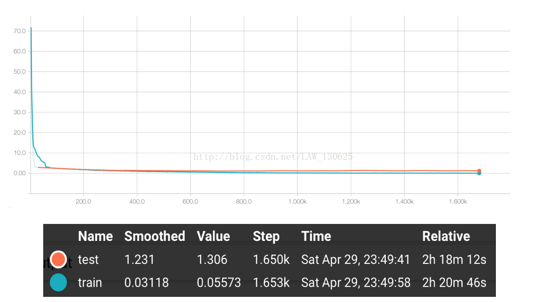
通过以上的训练,我们得到了最终结果的准确率大概在70%左右。具体的acurracy和loss走势可见如下使用TensorbBoard生成训练时记录下的数据的可视化图。
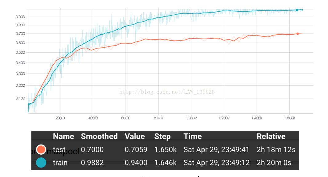
图2 accuracy
五、一些思考
本次实验的最好结果只有70.59%左右,并没有表现出AlexNet的强悍能力,综合分析主要有以下几个原因:
①观察上面图2的accuracy可以发现,在正确率上,前100个step中,测试集的效果比训练集的效果要好,但是之后测试集表现逐渐平缓,而训练集的效果继续逐渐上升,最后接近于1,所以可以推断最后模型出现了一定的过拟合,主要原因是AlexNet模型拟合能力强,而本次实验数据较为少,训练数据集只有1020个样本,所以模型出现了过拟合;
②在划分数据集上,可能存在个别类别的训练样本非常的少,所以难以训练出表现该类型的模型,自然而然模型效果也就差强人意;
③由于采用的是笔记本CPU进行训练模型,所以训练过程比较缓慢,因而基本没有进行太多的调参工作,如果仔细调参,模型应该还有上升的空间。


 1519
1519

 被折叠的 条评论
为什么被折叠?
被折叠的 条评论
为什么被折叠?
 到【灌水乐园】发言


