


Sharpening Spatial Filters
之前说到图像平滑/图像模糊使通过减少图像亮度剧烈变化的部分,可以采用像素值平均 (或加权平均),类似于积分。而锐化则强调亮度的转变,可以通过空间域像素的微分实现。微分算子的响应强度与该点出亮度不连续的程度成正比。因此,图像微分会增强边缘与其他不连续的成分 (如噪声),而不强调亮度缓慢变化的区域。平滑通常被称作低通滤波,而锐化又被称为高通滤波,即通过高频率的成分,而拒绝低频率的成分。总之,图像平滑是为了去除噪声,图像锐化则是增强图像边缘以及细节。
1、微分定义与性质
定义一元函数的一阶微分如下:
∂
f
∂
x
=
f
(
x
+
1
)
−
f
(
x
)
\frac{\partial f}{\partial x}=f(x+1)-f(x)
∂x∂f=f(x+1)−f(x)
我们可以将图像看成二元函数 f ( x , y ) f(x,y) f(x,y),根据上式可以获得关于 x x x或 y y y的一阶偏微分。
定义函数
f
(
x
)
f(x)
f(x)的二阶微分如下:
∂
2
f
∂
x
2
=
f
(
x
+
1
)
+
f
(
x
−
1
)
−
2
f
(
x
)
\frac{\partial^2 f}{\partial x^2}=f(x+1)+f(x-1)-2f(x)
∂x2∂2f=f(x+1)+f(x−1)−2f(x)
性质:
(1)一阶微分
亮度值为常数区域的一阶微分为0;
在斜坡内的一阶微分不为0;
在阶梯(向下斜坡)或斜坡(向上斜坡)处一阶微分不为0;
(2)二阶微分
亮度值为常数区域的二阶微分为0;
斜坡的二阶微分为0;
在转折点的二阶微分不为0;
Edges in digital images often are ramp-like transitions in intensity, in which case the first derivative of the image would result in thick edges because the derivative is nonzero along a ramp. On the other hand, the second derivative would produce a double edge one pixel thick, separated by zeros. From this, we conclude that the second derivative enhances fine detail much better than the first derivative, a property ideally suited for sharpening images. Also, second derivatives require fewer operations to implement than first derivatives, so our initial attention is on the former.
注意: 这里实际上是用差分代替微分。差分算子有前向差分、后向差分、中心差分。
前向差分:
f
′
(
x
)
≈
f
(
x
+
1
)
−
f
(
x
)
f^{'}(x) \approx f(x+1)-f(x)
f′(x)≈f(x+1)−f(x)
后向差分:
f
′
(
x
)
≈
f
(
x
)
−
f
(
x
−
1
)
f^{'}(x) \approx f(x)-f(x-1)
f′(x)≈f(x)−f(x−1)
中心差分:
f
′
(
x
)
≈
f
(
x
+
1
)
−
f
(
x
−
1
)
2
f^{'}(x) \approx \frac{f(x+1)-f(x-1)}{2}
f′(x)≈2f(x+1)−f(x−1)
2、二阶微分
最简单的各向同性(其响应与图像亮度不连续的方向无关)微分算子为Laplacian,定义拉普拉斯算子如下:
∇
2
f
=
∂
2
f
∂
x
2
+
∂
2
f
∂
y
2
\nabla^2 f=\frac{\partial^2 f}{\partial x^2}+\frac{\partial^2 f}{\partial y^2}
∇2f=∂x2∂2f+∂y2∂2f
由于任意阶微分都是线性运算,拉普拉斯也是线性算子。两个方向的二阶偏微分为:
∂
2
f
∂
x
2
=
f
(
x
+
1
,
y
)
+
f
(
x
−
1
,
y
)
−
2
f
(
x
,
y
)
\frac{\partial^2 f}{\partial x^2}=f(x+1,y)+f(x-1,y)-2f(x,y)
∂x2∂2f=f(x+1,y)+f(x−1,y)−2f(x,y)
∂ 2 f ∂ y 2 = f ( x , y + 1 ) + f ( x , y − 1 ) − 2 f ( x , y ) \frac{\partial^2 f}{\partial y^2}=f(x,y+1)+f(x,y-1)-2f(x,y) ∂y2∂2f=f(x,y+1)+f(x,y−1)−2f(x,y)
因此上述拉普拉斯算子改写为:
∇
2
f
(
x
,
y
)
=
f
(
x
+
1
,
y
)
+
f
(
x
−
1
,
y
)
+
f
(
x
,
y
−
1
)
+
f
(
x
,
y
+
1
)
−
4
f
(
x
,
y
)
\nabla^2 f(x,y)=f(x+1,y)+f(x-1,y)+f(x,y-1)+f(x,y+1)-4f(x,y)
∇2f(x,y)=f(x+1,y)+f(x−1,y)+f(x,y−1)+f(x,y+1)−4f(x,y)
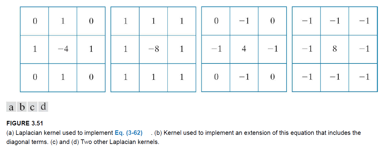
拉普拉斯是一个微分算子,它强调亮度的变化,而忽略亮度变化平缓的区域。这将倾向于产生具有灰色边缘线和其他不连续点的图像,所有这些都叠加在一个黑暗的、没有特征的背景上。为了恢复原始图像,同时保留拉普拉斯的锐化效果,需要将拉普拉斯滤波后的图像叠加到原图像上:
g
(
x
,
y
)
=
f
(
x
,
y
)
+
c
[
∇
2
f
(
x
,
y
)
]
g(x,y)=f(x,y)+c[\nabla^2 f(x,y)]
g(x,y)=f(x,y)+c[∇2f(x,y)]
g ( x , y ) g(x,y) g(x,y)为锐化图像。若拉普拉斯核的中心系数为负时, c = − 1 c=-1 c=−1;若拉普拉斯核的中心系数为正时, c = 1 c=1 c=1。
将拉普拉斯滤波后的图像添加到原图像,会增加亮度不连续区域(主要是边缘)的对比度,最终获得细节增强的图像同时保持背景色调。
In Section 3.5 , we normalized smoothing kernels so that the sum of their coefficients would be one. Constant areas in images filtered with these kernels would be constant also in the filtered image. We also found that the sum of the pixels in the original and filtered images were the same, thus preventing a bias from being introduced by filtering (see Problem 3.39 ). When convolving an image with a kernel whose coefficients sum to zero, it turns out that the pixels of the filtered image will sum to zero also (see Problem 3.40 ). This implies that images filtered with such kernels will have negative values, and sometimes will require additional processing to obtain suitable visual results. Adding the filtered image to the original, as we did in Eq. (3-63) , is an example of such additional processing.
在低通滤波时,我们对滤波核进行归一化处理,使得核的像素值之和为1;对于微分核,可以发现其滤波核的像素值之和为0。
3、Unsharp Masking and Highboost Filtering (非锐化掩蔽和高提升滤波)
unsharp masking (非锐化掩蔽): 通过从原图像中减去一个经过平滑(unsharp or smoothed)的图像获得一个掩模,然后令原图像加这个掩模来锐化图像。
g
m
a
s
k
(
x
,
y
)
=
f
(
x
,
y
)
−
f
ˉ
(
x
,
y
)
g_{mask}(x,y)=f(x,y)-\bar{f}(x,y)
gmask(x,y)=f(x,y)−fˉ(x,y)
g
(
x
,
y
)
=
f
(
x
,
y
)
+
k
g
m
a
s
k
(
x
,
y
)
g(x,y)=f(x,y)+kg_{mask}(x,y)
g(x,y)=f(x,y)+kgmask(x,y)
以上,当
k
=
1
k=1
k=1时,称为unsharp masking; 当
k
>
1
k>1
k>1时,称为highboost filtering。
4、一阶微分(梯度)
图像处理中的一阶微分是通过梯度的幅值来实现的。梯度定义如下:
∇
f
≡
g
r
a
d
(
f
)
=
[
g
x
g
y
]
=
[
∂
f
∂
x
∂
f
∂
y
]
\nabla f \equiv grad(f)= \left[ \begin{matrix} g_x \\ g_y \end{matrix} \right]= \left[ \begin{matrix} \frac{\partial f}{\partial x} \\ \frac{\partial f}{\partial y} \end{matrix} \right]
∇f≡grad(f)=[gxgy]=[∂x∂f∂y∂f]
梯度的物理意义为f在位置
(
x
,
y
)
(x,y)
(x,y)处变化最大的方向。
梯度的长度为:
M
(
x
,
y
)
=
∣
∣
∇
f
∣
∣
=
m
a
g
(
∇
f
)
=
g
x
2
+
g
y
2
M(x,y)=||\nabla f||=mag(\nabla f)=\sqrt{g_x^2+g_y^2}
M(x,y)=∣∣∇f∣∣=mag(∇f)=gx2+gy2
另外,常常用绝对值之和近似梯度:
M
(
x
,
y
)
≈
∣
g
x
∣
+
∣
g
y
∣
M(x,y) \approx |g_x|+|g_y|
M(x,y)≈∣gx∣+∣gy∣
注意,梯度是线性算子,梯度的长度不是线性算子。但梯度的长度是旋转不变的。
这里介绍三种一阶微分定义:
(1) 这是前面介绍过的,采用difference的定义
g x ( x , y ) = f ( x + 1 , y ) − f ( x , y ) g_x(x,y)=f(x+1,y)-f(x,y) gx(x,y)=f(x+1,y)−f(x,y)
g y ( x , y ) = f ( x , y + 1 ) − f ( x , y ) g_y(x,y)=f(x,y+1)-f(x,y) gy(x,y)=f(x,y+1)−f(x,y)
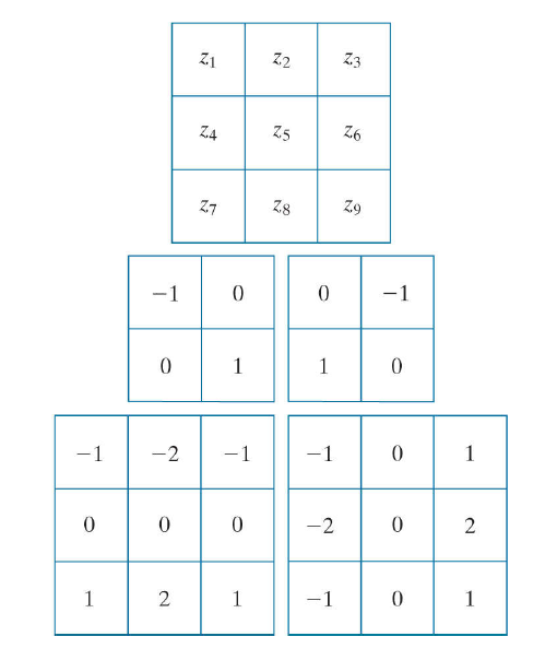
(2) Roberts 梯度算子
采用cross difference (如上图第二行的两个核),又称作Roberts cross-gradient operators。
g
x
(
x
,
y
)
=
f
(
x
+
1
,
y
+
1
)
−
f
(
x
,
y
)
g_x(x,y)=f(x+1,y+1)-f(x,y)
gx(x,y)=f(x+1,y+1)−f(x,y)
g y ( x , y ) = f ( x + 1 , y ) − f ( x , y + 1 ) g_y(x,y)=f(x+1,y)-f(x,y+1) gy(x,y)=f(x+1,y)−f(x,y+1)
(3) Sobel 算子
采用3*3的邻域,如上图的第三行。
g
x
(
x
,
y
)
=
∂
f
∂
x
=
(
f
(
x
+
1
,
y
−
1
)
+
2
f
(
x
+
1
,
y
)
+
f
(
x
+
1
,
y
+
1
)
)
−
(
f
(
x
−
1
,
y
−
1
)
+
2
f
(
x
−
1
,
y
)
+
f
(
x
−
1
,
y
+
1
)
)
g_x(x,y)=\frac{\partial f}{\partial x}=(f(x+1,y-1)+2f(x+1,y)+f(x+1,y+1))-(f(x-1,y-1)+2f(x-1,y)+f(x-1,y+1))
gx(x,y)=∂x∂f=(f(x+1,y−1)+2f(x+1,y)+f(x+1,y+1))−(f(x−1,y−1)+2f(x−1,y)+f(x−1,y+1))
g y ( x , y ) = ∂ f ∂ y = ( f ( x − 1 , y + 1 ) + 2 f ( x , y + 1 ) + f ( x + 1 , y + 1 ) ) − ( f ( x − 1 , y − 1 ) + 2 f ( x , y − 1 ) + f ( x + 1 , y − 1 ) ) g_y(x,y)=\frac{\partial f}{\partial y}=(f(x-1,y+1)+2f(x,y+1)+f(x+1,y+1))-(f(x-1,y-1)+2f(x,y-1)+f(x+1,y-1)) gy(x,y)=∂y∂f=(f(x−1,y+1)+2f(x,y+1)+f(x+1,y+1))−(f(x−1,y−1)+2f(x,y−1)+f(x+1,y−1))
从上图可以看出,一阶微分算子的元素之和为0,因此对于常亮度区域,其响应为0,另外若一幅图像与一个元素之和为0的卷积核进行卷积运算,其结果的元素之和为0。即结果图像存在负值。
梯度在工业检测中经常使用,要么是帮助人类检测缺陷,要么更常见的是作为自动化检测的预处理步骤。梯度可以用来增强缺陷并消除缓慢变化的背景特性。梯度的另一个重要特征是能够在平坦的灰度场中增强小的不连续点。
5、拉普拉斯算子(二阶)与梯度算子(一阶)的比较
The Laplacian, is a second-order derivative operator and has the definite advantage that it is superior for enhancing fine detail. However, this causes it to produce noisier results than the gradient. This noise is most objectionable in smooth areas, where it tends to be more visible. The gradient has a stronger response in areas of significant intensity transitions (ramps and steps) than does the Laplacian. The response of the gradient to noise and fine detail is lower than the Laplacian’s and can be lowered further by smoothing the gradient with a lowpass filter.
拉普拉斯算子用于增强细节,但是同时会产生噪声;梯度算子用于增强边缘,对于噪声与精细细节的响应较弱。


 204
204


 被折叠的 条评论
为什么被折叠?
被折叠的 条评论
为什么被折叠?
 到【灌水乐园】发言


