计算机视觉学习笔记（二）局部图像描述子

最新推荐文章于 2022-04-03 23:37:19 发布

coderJHT

最新推荐文章于 2022-04-03 23:37:19 发布

阅读量2.6k

点赞数

分类专栏：计算机视觉文章标签：计算机视觉

本文链接：https://blog.csdn.net/Lim11t/article/details/123854523

版权

计算机视觉专栏收录该内容

4 篇文章 1 订阅

订阅专栏

一、Harris角点检测器

1.1 角点检测算法原理

Harris 角点提取算法是Chris Harris 和Mike Stephens 在H.Moravec 算法的基础上发展出的通过自相关矩阵的角点提取算法，又称Plessey算法。Harris角点提取算法这种算子受信号处理中自相关面数的启发，给出与自相关函数相联系的矩阵M。M 阵的特征值是自相关函数的一阶曲率，如果两个曲率值都高，那么就认为该点是角点特征。
在这里插入图片描述
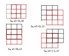
上图就是对Moravec算子的形象描述。用数学语言来表示的话就是：

其中（x，y）就表示四个移动方向（1，0）（1，1）（0，1）（-1，1），E就是像素的变化值。Moravec算子对四个方向进行加权求和来确定变化的大小，然和设定阈值，来确定到底是边还是角点。
Harris角点检测算子实质上就是对Moravec算子的改良和优化。在原文中，作者提出了三点Moravec算子的缺陷并且给出了改良方法：

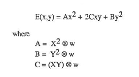
Moravec算子对方向的依赖性太强，在上文中我们可以看到，Moravec算子实际上只是移动了四个45度角的离散方向，真正优秀的检测算子应该能考虑到各个现象的移动变化情况。为此，作者采用微分的思想。

在这里插入图片描述
其中：

所以E就可以表示为：

1.2 角点检测相关概念

（1）特征点（兴趣点/关键点）
对于一幅图像，我们把目光从之前的观察整幅图像，转移到了图像中的某些特殊的点，对其进行分析。

如果能检测到足够的这种点，同时他们的区分度很高（可以精确定位稳定的特征），那么这个方法具有实用性。

特征点被大量的用于解决：物体识别、图像匹配、视觉跟踪、三维重建

图像特征类型被分为：边缘、角点（特征点）、斑点（特征区域）

（2）角点
角点通常被定义为两条边的交点，用术语的说法就是：在任意方向的一个微小变动都会引起灰度很大变化的点。

角点作为图像上的特征点，包含有重要的信息，在图像融合和目标跟踪及三维重建中有重要的应用价值，角点的描述也分为以下的三类：

一阶导数（即灰度的梯度）的局部最大所对应的像素点
两条及两条以上边缘的交点
图像中梯度值和梯度方向的变化速率都很高的点
角点的一阶导数最大、二阶导数为0、它指示了物体边缘变化不连续的方向

（3）角点检测

目前的角点检测算法可以归结为以下三类

基于灰度图的角点检测
基于二值图的角点检测
基于轮廓曲线的角点检测
基于灰度图的角点检测又可以分为基于梯度、基于模板和基于模板梯度组合的三类方法。

其中基于模板的方法主要考虑像素领域点的灰度变化，即图像亮度的变化，将与邻点亮度对比足够大的点定义为角点，Harris角点检测算法就是基于模板的角点检测方法。

1.3 响应函数

Harris角点检测器的响应函数会返回像素值为 Harris 响应函数值的一幅图像。

def compute_harris_response(im, sigma=3):
    """在一幅灰度图像中，对每个像素计算Harris角点检测器响应函数"""
    
    # 计算导数
    imx = zeros(im.shape)
    filters.gaussian_filter(im, (sigma, sigma), (0,1), imx)    
    imy = zeros(im.shape)
    filters.gaussian_filter(im, (sigma, sigma), (1,0), imy)
    
    # 计算Harris矩阵的分量
    Wxx = filters.gaussian_filter(imx*imx, sigma)
    Wxy = filters.gaussian_filter(imx*imy, sigma)
    Wyy = filters.gaussian_filter(imy*imy, sigma)
    
    # 计算特征值和迹
    Wdet = Wxx * Wyy - Wxy**2
    Wtr = Wxx + Wyy
    
    return Wdet / Wtr

将下面的函数添加到 harris.py 文件中：

def get_harris_points(harrisim, min_dist=10, threshold=0.1):
    """从一幅Harris响应图像中返回角点。min_dist为分割角点和图像边界的最小像素数目"""


    # 寻找高于阈值的候选角点
    corner_threshold = harrisim.max() * threshold
    harrisim_t = (harrisim > corner_threshold) * 1


    # 得到候选点的坐标
    coords = array(harrisim_t.nonzero()).T


    # 以及它们的Harris响应值
    candidate_values = [harrisim[c[0], c[1]] for c in coords]


    # 对候选点按照Harris响应值进行排序
    index = argsort(candidate_values)
    
    # 将可行点的位置保存到数组中
    allowed_locations = zeros(harrisim.shape)
    allowed_locations[min_dist:-min_dist,min_dist:-min_dist] = 1
    
    # 按照min_distance原则，选择最佳Harris点
    filtered_coords = []
    for i in index:
        if allowed_locations[coords[i,0], coords[i,1]] == 1:
            filtered_coords.append(coords[i])
            allowed_locations[(coords[i,0]-min_dist):(coords[i,0]+min_dist),
            (coords[i,1]-min_dist):(coords[i,1]+min_dist)] = 0
            
    return filtered_coords

1.4 Harris算法的优缺点

优点
旋转不变性，椭圆转过一定角度但是其形状保持不变（特征值保持不变）。
对于图像灰度的仿射变化具有部分的不变性，由于仅仅使用了图像的一介导数，对于图像灰度平移变化不变；
对于图像灰度尺度变化不变。
缺点
它对尺度很敏感，不具备几何尺度不变性。
提取的角点是像素级的

1.5 Harris算法代码实现

# -*- coding: utf-8 -*-
from pylab import *
from PIL import Image
from PCV.localdescriptors import harris


# 读入图像
im = array(Image.open('../JMU/grass.jpg').convert('L'))


# 检测harris角点
harrisim = harris.compute_harris_response(im)


# Harris响应函数
harrisim1 = 255 - harrisim


figure()
gray()


#画出Harris响应图
subplot(141)
imshow(harrisim1)
print (harrisim1.shape)
axis('off')
axis('equal')


threshold = [0.01,0.05,0.1]
for i, thres in enumerate(threshold):


    filtered_coords = harris.get_harris_points(harrisim, 6, thres)
    subplot(1, 4, i+2)
    imshow(im)
    print(im.shape)
    plot([p[1] for p in filtered_coords], [p[0] for p in filtered_coords], '*')
    axis('off')



show()

运行结果：
在这里插入图片描述

在这里插入图片描述
得到效果：

两张图像的匹配图像：

两张图片都是在尚大楼右侧，一张是远景，一张是从下往上拍的近照。
可以明显的发现有些特征匹配
由效果可见，哈里斯角点匹配对于集美大学中比较有特色的建筑里遇到了问题，准确度并不高！甚至说几乎大部分都是错误的。

二、SIFT

2.1 SIFT要解决的问题

目标的旋转、缩放、平移(RST)
图像仿射/投影变换(视点viewpoint )
弱光照影响( ilumination)
部分目标遮挡(occlusion)
杂物场景( clutter)
噪声

2.2 SIFT特性

特性独特性，也就是特征点可分辨性高，类似指纹，适合在海量数据中匹配。
多量性，提供的特征多。
高速性，就是速度快。
可扩展，能与其他特征向量联合使用。

2.3 尺度空间的概念

尺度空间是一个比较晦涩的概念，但尺度空间在自然空间中又是真是存在的，这里我们先从尺度谈起，在自然界物体都是由大小不同的实体组成，我们描述着些实体比如说房子、桌子一般会说有多高或者有多大，那么这个多高和多大一般所说就是长度和占地面积。在肉眼可见的情况下，我们常用厘米、米这样的标量尺度来描述长度和占地面积。而很少用纳米和微米这样很小的尺度。也就是说尺度是用来衡量一个量的一个标准。即我们可以用厘米来描述一个桌子多高，也可以用纳米来描述（当然生活中是没必要的）。
再来一个地图的例子，有世界地图和北京地图俩幅。在世界地图上（大尺度下）我们只能看到的是每一个国家的分布，但这个国家的仔细信息我们在这个尺度上是看不到的。但在北京地图上（小尺度下）我们就能清晰看出每一个街道或者商铺的名称。所以往往大尺度下关注的是物体的全局信息，如物体的轮廓等，小尺度下则更注重物体的细节。

以上，对现实中物体的描述一定要在一个十分重要的前提下进行，即对自然界建模时的尺度。当我们用一个机器视觉系统分析未知场景时，计算机没有办法预先知道图像中物体尺度，因此我们需要同时考虑图像在多尺度下的描述，获知感兴趣物体的最佳尺度。图像的尺度空间表达指的就是图像在所有尺度下的描述
在这里插入图片描述

2.4 代码实现


from PIL import Image
from pylab import *
from PCV.localdescriptors import sift
from PCV.localdescriptors import harris
import os



from matplotlib.font_manager import FontProperties
font = FontProperties(fname=r"d:\JsVison\font\SimSun.ttc", size=14)


imname = '../JMU/1.jpg'
im = array(Image.open(imname).convert('L'))
sift.process_image(imname, 'empire.sift')
l1, d1 = sift.read_features_from_file('empire.sift')




figure()
gray()
subplot(131)
sift.plot_features(im, l1, circle=False)
title(u'SIFT特征',fontproperties=font)
subplot(132)
sift.plot_features(im, l1, circle=True)
title(u'用圆圈表示SIFT特征尺度',fontproperties=font)


# 检测harris角点
harrisim = harris.compute_harris_response(im)


subplot(133)
filtered_coords = harris.get_harris_points(harrisim, 6, 0.1)
imshow(im)
plot([p[1] for p in filtered_coords], [p[0] for p in filtered_coords], '*')
axis('off')
title(u'imput image',fontproperties=font)

show()

运行结果：
在这里插入图片描述
找特征点：

找匹配点：

在这里可以发现，sift匹配也有错误，可能是由于对称，加上由于sift具有旋转不变特征，所以匹配的都是对称的点，或者有些是相似度极高的点。
这里我们可以发现，其实集美大学尚大楼这种比较有特色的建筑会给sift带来一些困难。但是不耽误它强大的匹配功能。虽说这几张图片效果不好。
再比较以下两张图：
在这里插入图片描述
总共209个匹配点。几乎没有匹配错的情况出现。

三、匹配地理标记图像

代码实现：

from pylab import *
from PIL import Image
from PCV.localdescriptors import sift
from PCV.tools import imtools
import pydot

""" This is the example graph illustration of matching images from Figure 2-10.
To download the images, see ch2_download_panoramio.py."""

#download_path = "panoimages"  # set this to the path where you downloaded the panoramio images
#path = "/FULLPATH/panoimages/"  # path to save thumbnails (pydot needs the full system path)

download_path = r"C:\Users\dell\Documents\VS_code workplace\SDL"  # set this to the path where you downloaded the panoramio images
path = r"C:\Users\dell\Documents\VS_code workplace\SDLsave"  # path to save thumbnails (pydot needs the full system path)

imlist = imtools.get_imlist(download_path)
nbr_images = len(imlist)

featlist = [imname[:-3] + 'sift' for imname in imlist]
for i, imname in enumerate(imlist):
    sift.process_image(imname, featlist[i])

matchscores = zeros((nbr_images, nbr_images))

for i in range(nbr_images):
    for j in range(i, nbr_images):  # only compute upper triangle
        print('comparing ', imlist[i], imlist[j])
        l1, d1 = sift.read_features_from_file(featlist[i])
        l2, d2 = sift.read_features_from_file(featlist[j])
        matches = sift.match_twosided(d1, d2)
        nbr_matches = sum(matches > 0)
        print('number of matches = ', nbr_matches)
        matchscores[i, j] = nbr_matches
print("The match scores is: \n", matchscores)
for i in range(nbr_images):
    for j in range(i + 1, nbr_images):  # no need to copy diagonal
        matchscores[j, i] = matchscores[i, j]

#可视化

threshold = 2  # min number of matches needed to create link

g = pydot.Dot(graph_type='graph')  # don't want the default directed graph

for i in range(nbr_images):
    for j in range(i + 1, nbr_images):
        if matchscores[i, j] > threshold:
            # first image in pair
            im = Image.open(imlist[i])
            im.thumbnail((100, 100))
            filename = path + str(i) + '.png'
            im.save(filename)  # need temporary files of the right size
            g.add_node(pydot.Node(str(i), fontcolor='transparent', shape='rectangle', image=filename))

            # second image in pair
            im = Image.open(imlist[j])
            im.thumbnail((100, 100))
            filename = path + str(j) + '.png'
            im.save(filename)  # need temporary files of the right size
            g.add_node(pydot.Node(str(j), fontcolor='transparent', shape='rectangle', image=filename))
            g.add_edge(pydot.Edge(str(i), str(j)))
g.write_png('jmu.png')

得到效果：
在这里插入图片描述

coderJHT

关注

0
点赞
踩
1

收藏

觉得还不错? 一键收藏
0
评论
计算机视觉学习笔记（二）局部图像描述子

目录一、Harris角点检测器1.1 角点检测算法原理1.2 角点检测相关概念1.3 响应函数1.4 Harris算法的优缺点1.5 Harris算法代码实现二、SIFT2.1 SIFT要解决的问题2.2 SIFT特性2.3 尺度空间的概念2.4 代码实现三、匹配地理标记图像一、Harris角点检测器1.1 角点检测算法原理Harris 角点提取算法是Chris Harris 和Mike Stephens 在H.Moravec 算法的基础上发展出的通过自相关矩阵的角点提取算法，又称Plessey算法。
复制链接

扫一扫