03_Classification_import name fetch_mldata_cross_val_plot_digits_ML_Project Checklist_confusion matr

handling multiple classes directly: Random Forest classifiers or naive Bayes classifiers

strictly binary classifiers: Support Vector Machine classifiers or Linear classifiers

Appendix B. Machine Learning Project Checklist
This checklist can guide you through your Machine Learning projects. There are eight main steps:
1. Frame the problem and look at the big picture.
2. Get the data.
3. Explore the data to gain insights.
4. Prepare the data to better expose the underlying data patterns to Machine Learning algorithms.
5. Explore many different models and short-list the best ones.
6. Fine-tune your models and combine them into a great solution.
7. Present your solution.
8. Launch, monitor, and maintain your system.
Obviously, you should feel free to adapt this checklist to your needs.

1. cross_val_predict(sgd_clf, X_train, y_train_5, cv=3)

from sklearn.model_selection import cross_val_predict

y_train_pred = cross_val_predict(sgd_clf, X_train, y_train_5, cv=3)

Just like the cross_val_score() function, cross_val_predict() performs K-fold cross-validation, but instead of returning the evaluation scores, it returns the predictions made on each test fold. This means that you get a clean prediction for each
instance in the training set (“clean” meaning that the prediction is made by a model that never saw the data during training).

from sklearn.metrics import confusion_matrix

confusion_matrix(y_train_5, y_train_pred)

		Predicted Class
		Class=No_(non_5s)_Negative	Class=Yes_Target(5s)_Positive
Actual Class	Class=No	TN	FP
	Class=Yes	FN	TP

             Non-5s      5s or Positive

from sklearn.metrics import precision_score, recall_score

precision_score(y_train_5, y_train_pred) #==3530/(3530+687) #TP/(TP+FP)

recall_score(y_train_5, y_train_pred) #==3530/(3530+1891) #TP/(TP+FN)

Each row in a confusion matrix represents an actual class, while each column represents a predicted class. The first row of this matrix considers non-5 images (the negative class): 53,892 of them were correctly classified as non-5s (they are called true negatives), while the remaining 687 were wrongly classified as 5s (false positives). The second row considers the images of 5s (the positive class): 1,891 were wrongly classified as non-5s (false negatives), while the remaining 3,530 were correctly classified as 5s (true positives). 

2. cross_val_predict(sgd_clf, X_train, y_train_5, cv=3, method="decision_function")

threshold? For this you will first need to get the scores of all instances in the training set using the cross_val_predict() function again, but this time specifying that you want it to return decision scores instead of predictions by setting method="decision_function":

#previously, #y_train_pred = cross_val_predict(sgd_clf, X_train, y_train_5, cv=3)
y_decision_scores = cross_val_predict(sgd_clf, X_train, y_train_5, cv=3, method="decision_function")

Now with these scores you can compute precision and recall for all possible thresholds using the precision_recall_curve() function:

from sklearn.metrics import precision_recall_curve

precisions, recalls, thresholds = precision_recall_curve(y_train_5, y_decision_scores)

3. cross_val_predict(forest_clf, X_train, y_train_5, cv=3, method="predict_proba")

the RandomForestClassifier class does not have a decision_function() method. Instead it has a predict_proba() method.

The predict_proba() method returns an array containing a row per instance and a column per class, each containing the probability that the given instance belongs to the given class (e.g., 70% chance that the image represents a 5):

from sklearn.ensemble import RandomForestClassifier

forest_clf = RandomForestClassifier(random_state=42)
y_probas_forest = cross_val_predict(forest_clf, X_train, y_train_5, cv=3, method="predict_proba")

#########################################beginning###############################

MNIST

we will be using the MNIST dataset, which is a set of 70,000 small images of digits handwritten by high school students and employees of the US Census Bureau. Each image is labeled with the digit it represents.

Scikit-Learn provides many helper functions to download popular datasets. MNIST is one of them. The following code fetches the MNIST dataset:

from sklearn.datasets import fetch_mldata

---------------------------------------------------------------------------
ImportError                               Traceback (most recent call last)
<ipython-input-1-f24642af8337> in <module>
----> 1 from sklearn.datasets import fetch_mldata

ImportError: cannot import name 'fetch_mldata'

Solution_1: #vesion-issue

# Python ≥3.5 is required
import sys
assert sys.version_info >= (3, 5)

# Scikit-Learn ≥0.20 is required
import sklearn
assert sklearn.__version__ >= "0.20"

from sklearn.datasets import fetch_openml
mnist = fetch_openml('mnist_784')
mnist.keys()

from collections import  Counter
Counter(mnist['target'])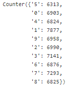

mnist

... ...

... ...

X, y = mnist["data"], mnist["target"]
X.shape

Solution_2:

from six.moves import urllib
from scipy.io import loadmat

mnist_url = "https://github.com/amplab/datascience-sp14/raw/master/lab7/mldata/mnist-original.mat"
mnist_datafile = "./mnist-original.mat" #saved filename in current directory

response = urllib.request.urlopen(mnist_url)
with open(mnist_datafile, 'wb') as f:
    content = response.read()
    f.write(content)

mnist_raw = loadmat(mnist_datafile)
mnist_raw

mnist_raw["data"].shape 

mnist_raw['label'].shape #from the result, we know each column has label in last row

mnist_raw["data"].T.shape 

mnist_raw['label'][0].shape #After data transpose and extraction, after the data columns is a label

mnist = {
    "COL_NAMES": ["label", "data"], #header
    'DESCR': 'mldata.org dataset: mnist-original',
    "data": mnist_raw["data"].T,
    "target": mnist_raw["label"][0],
}
mnist.keys()

Datasets loaded by Scikit-Learn generally have a similar dictionary structure including:
• A DESCR key describing the dataset
• A data key containing an array with one row per instance and one column per feature
• A target key containing an array with the labels

X, y = mnist["data"], mnist["target"]
X.shape

y.shape

mnist['feature_names'][-1]

There are 70,000 images, and each image has 784 features. This is because each image is 28×28 pixels, and each feature simply represents one pixel’s intensity像素, from 0 (white) to 255 (black). Let’s take a peek看一眼 at one digit from the dataset. All you need to do is grab an instance’s feature vector, reshape it to a 28×28 array, and display it using Matplotlib’s imshow() function:

%matplotlib inline
import matplotlib
import matplotlib.pyplot as plt

some_digit = X[0] #784=28*28

some_digit_image = some_digit.reshape(28,28)
plt.imshow(some_digit_image, cmap = matplotlib.cm.binary, interpolation="nearest")
plt.axis("off")

plt.show()

This looks like a 5, and indeed that’s what the label tells us:

y[0]

#you also can use the following code

import matplotlib as mpl
y=y.astype(np.uint8)
def plot_digit(data):
    image = data.reshape(28,28)
    plt.imshow(image, cmap=mpl.cm.binary, interpolation="nearest")
    plt.axis("off")
    plt.show()
plot_digit(X[0])

Following figure shows a few more images from the MNIST dataset to give you a feel for the complexity of the classification task.

#Extra
import matplotlib as mpl
    
def plot_digits(instances, images_per_row=10, **options):
    size = 28
    images_per_row = min(len(instances), images_per_row)
    n_rows = (len(instances)-1) //images_per_row + 1#or (49-1)//10+1=5 instead 49//10=4 : need +1
                                                    #or (52-1)//10+1=6 instead 52//10=5 # need +1
                                                    #or (50-1)//10+1=5 instead (50)//10+1=6 need 50-1
    images = [eachInstance.reshape(size,size) for eachInstance in instances] #ndarray
    row_images=[]
    #process empty on the last row or the number of last row images != images_per_row
    if n_rows * images_per_row >len(instances) : #fill with 28*28 0's
        n_empty = n_rows * images_per_row -len(instances)
                               #hint:tile horizontal                           #Dimension
        images.append(np.zeros((size,size*n_empty))#wrong:np.zeros((size,size))*n_empty==np.zeros((size,size))
                     )                      #wrong:np.zeros((size,size)*n_empty) #2^n_empty dimensions
#OR
#         images.append(np.tile(np.zeros((size,size)),n_empty)
#                      ) 
    #print(len(images)) #check previous if statement
    #images: [array, array...,array]
    #in each array
    #print(len(images[0][0])) #28 columns
    #print(len(images[0]))    #28 rows

    for row in range(n_rows):        #index[0]  : image[0]...image[9] in row 0
        rimages = images[row*images_per_row: (row+1)*images_per_row] #block or subgroup
        row_images.append(np.concatenate(rimages, axis=1)) #images per row
    images= np.concatenate(row_images, axis=0)
                          
    plt.imshow(images, cmap=mpl.cm.binary, **options)
    plt.axis("off") 


plt.figure(figsize=(9,9))
example_images = X[:100]
plot_digits(example_images, images_per_row=10)
plt.show()       

But wait! You should always create a test set and set it aside before inspecting the data closely. The MNIST dataset is actually already split into a training set (the first 60,000 images) and a test set (the last 10,000 images):

Note: we don't need do stratified sampling
(02_End-to-End Machine Learning Project: https://blog.csdn.net/Linli522362242/article/details/103387527)

X_train, X_test, y_train, y_test = X[:60000], X[60000:], y[:60000], y[60000:]

Let’s also shuffle the training set; this will guarantee that all cross-validation folds will be similar (you don’t want one fold to be missing some digits). Moreover, some learning algorithms are sensitive to the order of the training instances, and they perform poorly if they get many similar instances in a row.
Shuffling the dataset ensures that this won’t happen:

shuffle_index = np.random.permutation(len(X_train)) #len(X_train) ==60000
X_train, y_train = X_train[shuffle_index], y_train[shuffle_index]

X_train, X_test, y_train, y_test = X[:60000], X[60000:], y[:60000], y[60000:] #for tracking the steps

 Training a Binary Classifier

Let’s simplify the problem for now and only try to identify one digit — for example, the number 5. This “5-detector” will be an example of a binary classifier, capable of distinguishing between just two classes, 5 and not-5. Let’s create the target vectors for this classification task:

y_train_5 = (y_train==5)
y_test_5 = (y_test==5)

y_train_5

y_test_5

Okay, now let’s pick a classifier and train it. A good place to start is with a Stochastic Gradient Descent
(SGD) classifier, using Scikit-Learn’s SGDClassifier class. This classifier has the advantage of being capable of handling very large datasets efficiently. This is in part because SGD deals with training instances independently, one at a time (which also makes SGD well suited for online learning), as we will see later. Let’s create an SGDClassifier and train it on the whole training set:

###############
Tip: The SGDClassifier relies on randomness during training (hence the name “stochastic”). If you want reproducible results, you should set the random_state parameter.
###############

1.##############Training Classifier ##############

from sklearn.linear_model import SGDClassifier
                                                         #0.001
sgd_clf = SGDClassifier(random_state=42, max_iter=1000, tol=1e-3)
sgd_clf.fit(X_train, y_train_5)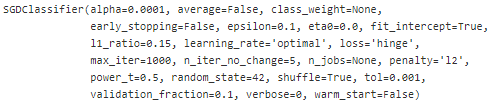

sgd_clf.predict([some_digit]) #detect images of the number 5

The classifier guesses that this image represents a 5 (True). Looks like it guessed right in this particular case! Now, let’s evaluate this model’s performance.

Performance Measures         2.choose the appropriate metric for your task

Evaluating a classifier回归器 is often significantly trickier复杂的 than evaluating a regressor回归器, so we will spend a largepart on this topic. There are many performance measures available, so grab another coffee and get ready to learn many new concepts and acronyms 首字母缩略词!

Measuring Accuracy Using Cross-Validation

Let’s use the cross_val_score() function to evaluate your SGDClassifier model using K-fold crossvalidation, with three folds. Remember that K-fold cross-validation means splitting the training set into K-folds (in this case, three), then making predictions and evaluating them on each fold using a model trained on the remaining folds.

from sklearn.model_selection import cross_val_score
cross_val_score(sgd_clf, X_train, y_train_5, cv=3, scoring='accuracy')

################################################################

T: True prediction or classify correctly;     F: False prediction or classify incorrectly
P: instance is truely belong to target class based on the fact;     
N: instance is not belong to target class based on the fact
Accuracy = (TP+TN)/(TP+FP+FN+TN)
Precision = TP/(TP+FP) # True predicted/ (True predicted + False predicted)
Recall = TP/(TP+FN)

https://towardsdatascience.com/accuracy-recall-precision-f-score-specificity-which-to-optimize-on-867d3f11124

A school is running a machine learning primary diabetes scan on all of its students.
The output is either diabetic (+ve) (Target)or healthy (-ve)(Not Target).

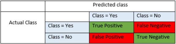
There are only 4 cases any student X could end up with.
We’ll be using the following as a reference later, So don’t hesitate to re-read it if you get confused.

• True positive (TP): Prediction is +ve and X is diabetic, we want that: true positive is a diabetic person(Target) correctly predicted(You believed) .
• True negative (TN): Prediction is -ve and X is healthy, we want that too: true negative is a healthy person(Not Target) correctly predicted(You believed) 
• False positive (FP): Prediction is +ve and X is healthy, false alarm, bad: false positive is a healthy person(Not target) incorrectly predicted as diabetic(+) 
• False negative (FN): Prediction is -ve and X is diabetic, the worst.: false negative is a diabetic person(target) incorrectly predicted as healthy(-)

Which performance metric to choose?

Accuracy

It’s the ratio of the correctly labeled subjects to the whole pool of subjects.
Accuracy is the most intuitive最直观的  one.
Accuracy answers the following question: How many students did we correctly label out of all the students? 
Accuracy = (TP+TN)/(TP+FP+FN+TN)
numerator: all correctly labeled subject (All trues)
denominator: all subjects

Precision

Precision is the ratio of the correctly +ve labeled by our program to all +ve labeled.
Precision answers the following: How many of those who we (target)labeled as diabetic are actually diabetic?
Precision = TP/(TP+FP) # True predicted/ (True predicted + False predicted)
numerator: +ve labeled diabetic people.
denominator: all +ve (actually diabetic) labeled by our program (whether they’re diabetic or not in reality).

Recall (aka Sensitivity)

Recall is the ratio of the correctly +ve labeled by our program to all who are diabetic in reality.
Recall answers the following question: Of all the people who are diabetic(target), how many of those we correctly predict?
Recall = TP/(TP+FN)
numerator: +ve labeled diabetic people.
denominator: all people who are diabetic (whether detected by our program or not)

F1-score (aka F-Score / F-Measure)

F1 Score considers both precision and recall.
It is the harmonic mean(average) of the precision and recall.
F1 Score is best if there is some sort of balance between precision (p) & recall (r) in the system. Oppositely F1 Score isn’t so high if one measure is improved at the expense of the other. 
For example, if P is 1 & R is 0, F1 score is 0.
F1 Score = 2*(Recall * Precision) / (Recall + Precision)

Specificity or called TNR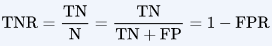

Specificity is the correctly -ve labeled by the program to all who are healthy in reality.
Specifity answers the following question: Of all the people who are healthy(Not target), how many of those did we correctly predict?
Specificity = TN/(TN+FP)
numerator: -ve labeled healthy people.
denominator: all people who are healthy in reality (whether +ve or -ve labeled)

General Notes

Yes, accuracy is a great measure but only when you have symmetric datasets (false negatives & false positives counts are close), also, false negatives & false positives have similar costs.
If the cost of false positives and false negatives are different then F1 is your savior. F1 is best if you have an uneven class distribution.

Precision is how sure you are of your true positives whilst recall is how sure you are that you are not missing any positives.

Bottom Line is

— Accuracy value of 90% means that 1 of every 10 labels is incorrect, and 9 is correct.
— Precision value of 80% means that on average, 2 of every 10 diabetic(target) labeled student by our program is healthy, and 8 is diabetic(target).
— Recall value is 70% means that 3 of every 10 diabetic people (target) in reality are missed by our program and 7 labeled as diabetic.
— Specificity value is 60% means that 4 of every 10 healthy people(Not target) in reality are miss-labeled as diabetic and 6 are correctly labeled as healthy.

################################################################
IM PLEM ENTING CROSS-VALIDATION
Occasionally you will need more control over the cross-validation process than what Scikit-Learn provides off-the-shelf. In these cases, you can implement cross-validation yourself; it is actually fairly straightforward. The following code does roughly the same thing as Scikit-Learn’s cross_val_score() function, and prints the same result:

from sklearn.model_selection import StratifiedKFold
from sklearn.base import clone

skfolds = StratifiedKFold(n_splits=3, random_state=42)#if error, set shuffle = False. 

for train_index, test_index in skfolds.split(X_train, y_train_5):
    clone_clf = clone(sgd_clf)    #sgd_clf = SGDClassifier(random_state=42, max_iter=1000, tol=1e-3)
    X_train_folds = X_train[train_index]
    y_train_folds = y_train_5[train_index]
    X_test_fold = X_train[test_index]
    y_test_fold = y_train_5[test_index]
    
    clone_clf.fit(X_train_folds, y_train_folds)
    y_pred = clone_clf.predict(X_test_fold)
    n_correct = sum(y_pred==y_test_fold)
    print(n_correct/len(y_test_fold))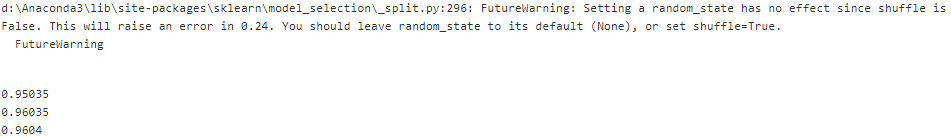

https://blog.csdn.net/Linli522362242/article/details/103387527
The StratifiedKFold class performs stratified sampling to produce folds that contain a representative ratio of each class. At each iteration the code creates a clone of the classifier, trains that clone on the training folds, and makes predictions on the test fold. Then it counts the number of correct predictions and outputs the ratio of correct predictions.

################################################################

from sklearn.model_selection import cross_val_score
cross_val_score(sgd_clf, X_train, y_train_5, cv=3, scoring='accuracy')

Wow! Above 95% accuracy (ratio of correct predictions) on all cross-validation folds? This looks amazing, doesn’t it? Well, before you get too excited, let’s look at a very dumb笨 classifier that just classifies every single image in the “not-5” class:

from sklearn.base import BaseEstimator

class Never5Classifier(BaseEstimator):
    def fit(self, X, y=None):
        pass
    def predict(self, X):
        return np.zeros((len(X), 1), dtype=bool)

never_5_clf = Never5Classifier()
cross_val_score(never_5_clf, X_train, y_train_5, cv=3, scoring="accuracy")

That’s right, it has over 90% accuracy! This is simply because only about 10% of the images are 5s, so if you always guess that an image is not a 5, you will be right about 90% of the time. Beats Nostradamus諾斯塔達摩斯.
This demonstrates why accuracy is generally not the preferred performance measure for classifiers, especially when you are dealing with skewed datasets (i.e., when some classes are much more frequent than others).

3. Confusion Matrix混淆矩阵 ####evaluate your classifiers using cross-validation####

A much better way to evaluate the performance of a classifier is to look at the confusion matrix. The general idea is to count the number of times instances of class A are classified as class B. For example, to know the number of times the classifier confused images of 5s with 3s, you would look in the 5th row and 3rd column of the confusion matrix.

To compute the confusion matrix, you first need to have a set of predictions, so they can be compared to the actual targets. You could make predictions on the test set, but let’s keep it untouched for now (remember that you want to use the test set only at the very end of your project, once you have a classifier that you are ready to launch). Instead, you can use the cross_val_predict() function:

from sklearn.model_selection import cross_val_predict

y_train_pred = cross_val_predict(sgd_clf, X_train, y_train_5, cv=3)

Just like the cross_val_score() function, cross_val_predict() performs K-fold cross-validation, but instead of returning the evaluation scores, it returns the predictions made on each test fold. This means that you get a clean prediction for each
instance in the training set (“clean” meaning that the prediction is made by a model that never saw the data during training).

Now you are ready to get the confusion matrix using the confusion_matrix() function. Just pass it the target classes (y_train_5) and the predicted classes (y_train_pred):

from sklearn.metrics import confusion_matrix

confusion_matrix(y_train_5, y_train_pred)

		Predicted Class
		Class=No_(non_5s)_Negative	Class=Yes_Target(5s)_Positive
Actual Class	Class=No	TN	FP
	Class=Yes	FN	TP

             Non-5s      5s or Positive

Each row in a confusion matrix represents an actual class, while each column represents a predicted class. The first row of this matrix considers non-5 images (the negative class): 53,892 of them were correctly classified as non-5s (they are called true negatives), while the remaining 687 were wrongly classified as 5s (false positives). The second row considers the images of 5s (the positive class): 1,891 were wrongly classified as non-5s (false negatives), while the remaining 3,530 were correctly classified as 5s (true positives). A perfect classifier would have only true positives 687and true negatives, so its confusion matrix would have nonzero values only on its main diagonal (top left to bottom right):

y_train_perfect_predictions = y_train_5 #pretend we reached perfection
confusion_matrix(y_train_5, y_train_perfect_predictions)

The confusion matrix gives you a lot of information, but sometimes you may prefer a more concise metric. An interesting one to look at is the accuracy of the positive predictions; this is called the precision of the classifier.

TP is the number of true positives, and FP is the number of false positives

A trivial way to have perfect precision is to make one single positive prediction and ensure it is correct (precision = 1/1 = 100%). This would not be very useful since the classifier would ignore all but one positive instance. So precision is typically used along with another metric named recall, also called sensitivity or true positive rate (TPR): this is the ratio of positive instances that are correctly detected by the classifier

FN is of course the number of false negatives.

If you are confused about the confusion matrix, Figure 3-2 may help.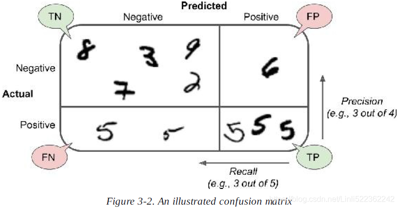

Precision and Recall

Scikit-Learn provides several functions to compute classifier metrics, including precision and recall

from sklearn.metrics import precision_score, recall_score

precision_score(y_train_5, y_train_pred) #==3530/(3530+687)

3530/(3530+687)#TP/(TP+FP)

recall_score(y_train_5, y_train_pred) #==3530/(3530+1891)

3530/(3530+1891)#TP/(TP+FN)

Now your 5-detector does not look as shiny as it did when you looked at its accuracy. When it claims an
image represents a 5, it is correct only 84%(0.8370879772350012) of the time. Moreover, it only detects 65% of the 5s.

It is often convenient to combine precision and recall into a single metric called the F1 score, in particular if you need a simple way to compare two classifiers. The F1 score is the harmonic mean of precision and recall (Equation 3-3). Whereas the regular mean treats all values equally, the harmonic调和的mean gives much more weight to low values. As a result, the classifier will only get a high F1 score if both recall and precision are high.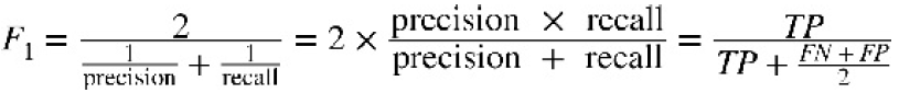

To compute the F1 score, simply call the f1_score() function:

from sklearn.metrics import f1_score

f1_score(y_train_5, y_train_pred)

4. ##############select the precision/recall tradeoff that fits your needs##

The F1 score favors classifiers that have similar precision and recall. This is not always what you want: in some contexts you mostly care about precision, and in other contexts you really care about recall. For example, if you trained a classifier to detect videos that are safe for kids, you would probably prefer a classifier that rejects many good videos (low recall) but keeps only safe ones (high precision), rather than a classifier that has a much higher recall but lets a few really bad videos show up in your product (in such cases, you may even want to add a human pipeline to check the classifier’s
video selection).

:  True / False means Is the classification correct； P means whether the class to which the object(instance in each row of dataset) belongs is the target class(videos that are safe for kids); you expect high precision. FP: the rate of missclassifying(F) other kinds of videos as the target class(P); FN: the rate of missclassifying(F) the viedos that are safe for kids as other kinds of videos. you more care about FP.

On the other hand, suppose you train a classifier to detect shoplifters扒手 on surveillance images监控影像: it is probably fine if your classifier has only 30% precision as long as it has 99% recall (sure, the security guards will get a few false alerts, but almost all shoplifters will get caught).

: True / False means Is the classification correct； P means whether the class to which the object(instance in each row of dataset) belongs is the target class(shoplifter) or the non-target class(Good customer); you expect high recall rate since you want all most shoplifters will be get caught by the security guards and few shoplifters are wrongly(F) classfied as non-target class(Good customer, N). FP：the rate of Misclassifying(F) good customers as shoplifters(P), FN and FP, you more care about FN.

Unfortunately, you can’t have it both ways: increasing precision reduces recall, and vice versa. This is called the precision/recall tradeoff.

Precision/Recall Tradeoff

To understand this tradeoff, let’s look at how the SGDClassifier makes its classification decisions. For each instance, it computes a score based on a decision function, and if that score is greater than a threshold, it assigns the instance to the positive class(Target), or else it assigns it to the negative class(Non-target). Figure 3-3 shows a few digits positioned
from the lowest score on the left to the highest score on the right. Suppose the decision threshold is positioned at the central arrow (between the two 5s): you will find 4 true positives (actual four 5s) on the right of that threshold, and one false positive (actually a 6). Therefore, with that threshold, the precision is 80% (4 out of 5 =(4/(4+1)=TP/(TP+FP) ). But (total is six 5s)out of 6 actual 5s, the classifier only detects 4, so the recall is 67% (4 out of 6(=4/(4+2)=TP/(TP+FN))).

Now if you raise the threshold (move it to the arrow on the right), the false positive (the 6) becomes a true negative, thereby increasing precision (up to 100%=3/(3+0) in this case), but one true positive becomes a false negative, decreasing recall down to 50%=3/(3+3).

Conversely, lowering the threshold increases recall and reduces precision.

Scikit-Learn does not let you set the threshold directly, but it does give you access to the decision scores that it uses to make predictions. Instead of calling the classifier’s predict() method, you can call its decision_function() method, which returns a score for each instance, and then make predictions based on those scores using any threshold you want:

y_decision_scores = sgd_clf.decision_function([some_digit])
y_decision_scores

threshold=0
y_some_digit_pred = (y_decision_scores > threshold)
y_some_digit_pred

The SGDClassifier uses a threshold equal to 0, so the previous code returns the same result(True) as the predict() method (i.e., True). Let’s raise the threshold to 200000:

threshold=200000
y_some_digit_pred = (y_decision_scores>threshold)
y_some_digit_pred

This confirms that raising the threshold decreases recall. The image actually represents a 5, and the classifier detects it when the threshold is 0, but it misses it when the threshold is increased to 200,000.

So how can you decide which threshold to use? For this you will first need to get the scores of all instances in the training set using the cross_val_predict() function again, but this time specifying that you want it to return decision scores instead of predictions by setting method="decision_function":

4. ##############select the precision/recall tradeoff that fits your needs##############

#previously, #y_train_pred = cross_val_predict(sgd_clf, X_train, y_train_5, cv=3)
y_decision_scores = cross_val_predict(sgd_clf, X_train, y_train_5, cv=3, method="decision_function")

Now with these scores you can compute precision and recall for all possible thresholds using the precision_recall_curve() function:

from sklearn.metrics import precision_recall_curve

precisions, recalls, thresholds = precision_recall_curve(y_train_5, y_decision_scores)

Finally, you can plot precision and recall as functions of the threshold value using Matplotlib

%matplotlib inline
import matplotlib as mpl
import matplotlib.pyplot as plt

def plot_precision_recall_vs_threshold(precisions, recalls, thresholds):
    plt.plot(thresholds, precisions[:-1], 'b--', label="Precision")
    plt.plot(thresholds, recalls[:-1], 'g-', label="Recall")
    plt.xlabel("Threshold", fontsize=16)
    #plt.ylim([0,1])
    plt.legend(loc="upper left", fontsize=16)
    plt.grid(True)           #plt.ylim([0,1])
    plt.axis([-50000, 50000, 0,1])
    plt.title('Figure 3-4.Precision and recall versus the decision threshold')

plt.figure(figsize=(8,4))    
plot_precision_recall_vs_threshold(precisions, recalls, thresholds)
plt.plot([7813, 7813], [0., 0.93],"r:")
plt.plot([-50000, 7813], [0.93, 0.93], "r:")
plt.plot([7813], [0.93], "ro")
plt.plot([-50000, 7813], [0.3068, 0.3068], "r:")
plt.plot([7813], [0.3068], "ro")

plt.show()

#######################################################

NOTE
You may wonder why the precision curve is bumpier崎岖的 than the recall curve in Figure 3-4. The reason is that precision may
sometimes go down when you raise the threshold (although in general it will go up). To understand why, look back at Figure 3-3
and notice what happens when you start from the central threshold and move it just one digit to the right: precision goes from 4/5 (80%) down to 3/4 (75%). On the other hand, recall can only go down when the threshold is increased, which explains why its curve looks smooth.

(y_train_pred == (y_decision_scores >0)).all()

     #not exists missing value
#######################################################

Now you can simply select the threshold value that gives you the best precision/recall tradeoff for your task. Another way to select a good precision/recall tradeoff is to plot precision directly against recall, as shown in Figure

def plot_precision_vs_recall(precisions, recalls):
    plt.plot(recalls, precisions, "b-", lw=2)
    plt.xlabel("Recall", fontsize=16)
    plt.ylabel("Precision", fontsize=16)
    plt.axis([0,1, 0,1])
    plt.grid(True)
    
plt.figure(figsize=(8,6))
plot_precision_vs_recall(precisions, recalls)
plt.plot([0.3068, 0.3068], [0., 0.93], "r:")
plt.plot([0.0, 0.3068], [0.93, 0.93], "r:")
plt.plot([0.3068], [0.93], "ro")
plt.title("Precision versus recall")

plt.show()

4. ##############select the precision/recall tradeoff that fits your needs##

You can see that precision really starts to fall sharply around 80% recall. You will probably want to select a precision/recall tradeoff just before that drop — for example, at around 60% recall. But of course the choice depends on your project.

So let's suppose you decide to aim for 93% precision. You look up the first plot (zooming in a bit) and find that you need to use a threshold of about 70,000. To make predictions (on the training set for now), instead of calling the classifier's predict() method, you can just run this code:

The index of precisions corresponds to the index of thresholds, so we need to get the index of our precision value(0.93), then we get the threshold value through this index, finally  we can get the specified precision score and recall score(rate) . 

threshold_93_precision=thresholds[np.argmax(precisions>=0.93)]
print(threshold_93_precision)

y_train_pred_93 = (y_decision_scores>=threshold_93_precision)
y_train_pred_93

precision_score(y_train_5, y_train_pred_93)

recall_score(y_train_5, y_train_pred_93)

Great, you have a 93% precision classifier (or close enough)! As you can see, it is fairly easy to create a classifier with virtually any precision you want: just set a high enough threshold, and you’re done. Hmm, not so fast. A high-precision classifier is not very useful if its recall is too low!
####################################################
TIP
If someone says “let’s reach 99% precision,” you should ask, “at what recall?”
####################################################

https://en.wikipedia.org/wiki/Sensitivity_and_specificity
The ROC Curve(TPr / FPr = 1-TNr)

The receiver operating characteristic (ROC) curve 接收器工作特性曲线is another common tool used with binary classifiers. It is very similar to the precision / recall curve, but instead of plotting precision versus recall,
the ROC curve plots the true positive rate (another name for recall) against the false positive rate(TPR vs FPR).
The FPR is the ratio of negative instances that are incorrectly classified as positive. It is equal to one minus the true negative rate(FPR=1-TNR),
the true negative rate,which is the ratio of negative instances that are correctly classified as negative. The TNR is also called specificity. Thus the ROC curve plots sensitivity (recall) versus 1 – specificity(TNR).

To plot the ROC curve, you first need to compute the TPR and FPR for various threshold values, using the roc_curve() function:

5. ##############compare various models using ROC curves ##############

from sklearn.metrics import roc_curve

#y_decision_scores = cross_val_predict(sgd_clf, X_train, y_train_5, cv=3, method="decision_function")
fpr, tpr, thresholds = roc_curve(y_train_5, y_decision_scores)

def plot_roc_curve(fpr, tpr, label=None):
    plt.plot(fpr, tpr, lw=2, label=label)
    plt.plot([0,1], [0,1], 'k--') #dashed diagnoal
    plt.axis([0,1,0,1])
    plt.xlabel("False Positive Rate (Fall-Out)", fontsize=16)
    plt.ylabel("True Positive Rate (Recall)", fontsize=16)
    plt.grid(True)
        
plt.figure(figsize=(8,6))
plot_roc_curve(fpr, tpr)
plt.plot([4.837e-3, 4.837e-3], [0.0, 0.3068], 'y:')
plt.plot([4.837e-3], [0.3068],'yo')
plt.show()

Once again there is a tradeoff: the higher the recall (TPR), the more false positives (FPR) the classifier produces. The dotted line represents the ROC curve of a purely random classifier; a good classifier stays as far away from that line as possible (toward the top-left corner).

One way to compare classifiers is to measure the area under the curve (AUC). A perfect classifier will have a ROC AUC equal to 1, whereas a purely random classifier will have a ROC AUC equal to 0.5. Scikit-Learn provides a function to compute the ROC AUC:

from sklearn.metrics import roc_auc_score

roc_auc_score(y_train_5, y_decision_scores)

#######################################
TIP
Since the ROC curve is so similar to the precision/recall (or PR) curve, you may wonder how to decide which one to use. As a
rule of thumb, you should prefer the PR curve whenever the positive class(target) is rare or when you care more about the false positives than the false negatives, and the ROC curve otherwise. For example, looking at the previous ROC curve (and the ROC AUC score), you may think that the classifier is really good. But this is mostly because there are few positives (5s) compared to the negatives (non-5s). In contrast, the PR curve makes it clear that the classifier has room for improvement (the curve could be closer to the top-right corner).
#######################################
Let’s train a RandomForestClassifier and compare its ROC curve and ROC AUC score to the SGDClassifier. First, you need to get scores for each instance in the training set. But due to the way it works, the RandomForestClassifier class does not have a decision_function() method. Instead it has a predict_proba() method. Scikit-Learn classifiers generally have one or the
other. The predict_proba() method returns an array containing a row per instance and a column per class, each containing the probability that the given instance belongs to the given class (e.g., 70% chance that the image represents a 5):

#we set n_estimators=100 to be future-proof since this will be the default value in Scikit-Learn 0.22
forest_clf = RandomForestClassifier(random_state=42, n_estimators=100)
y_probas_forest = cross_val_predict(forest_clf, X_train, y_train_5, cv=3, method="predict_proba")

y_probas_forest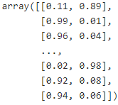

But to plot a ROC curve, you need scores, not probabilities. A simple solution is to use the positive class’s probability as the score; Now you are ready to plot the ROC curve. It is useful to plot the first ROC curve as well to see how they
compare

5. ##############compare various models using ROC curves ##############

y_scores_forest = y_probas_forest[:,1] #score = proba of positive class
fpr_forest, tpr_forest, thresholds_forest = roc_curve(y_train_5, y_scores_forest)

plt.figure(figsize=(8,6))
plt.plot(fpr,tpr, "b:", lw=2, label="SGD") #Stochastic Gradient Descent(SGD) classifier
plot_roc_curve(fpr_forest, tpr_forest, "Random_Forest")

plt.grid(True)
plt.legend(loc="lower right", fontsize=16)
plt.title('Comparing ROC curves')
plt.show()

As you can see in Figure, the RandomForestClassifier’s ROC curve looks much better than the SGDClassifier’s: it comes much closer to the top-left corner. As a result, its ROC AUC score is also significantly better:

6. ##############ROC AUC scores ##############

roc_auc_score(y_train_5, y_scores_forest) #y_probas_forest[:,1] #score = proba of positive class

Try measuring the precision and recall scores: you should find 98.5% precision and 82.8% recall. Not
too bad!

y_train_pred_forest = cross_val_predict(forest_clf, X_train, y_train_5, cv=3)
precision_score(y_train_5, y_train_pred_forest)

recall_score(y_train_5, y_train_pred_forest)

Hopefully you now know how to 1.train binary classifiers, 2.choose the appropriate metric for your task(accuracy), 3.evaluate your classifiers using cross-validation(confusion matrix), 4.select the precision/recall tradeoff that fits your needs, and 5.compare various models using ROC curves and 6..ROC AUC scores. Now let’s try to detect more than just the 5s.

Multiclass Classification

Whereas binary classifiers distinguish between two classes, multiclass classifiers (also called multinomial classifiers) can distinguish between more than two classes.

Some algorithms (such as Random Forest classifiers or naive Bayes classifiers) are capable of handling multiple classes directly. Others (such as Support Vector Machine classifiers or Linear classifiers) are strictly binary classifiers. However, there are various strategies that you can use to perform multiclass classification using multiple binary classifiers.

For example, one way to create a system that can classify the digit images into 10 classes (from 0 to 9) is to train 10 binary classifiers, one for each digit (a 0-detector, a 1-detector, a 2-detector, and so on). Then when you want to classify an image, you get the decision score from each classifier for that image and you select the class whose classifier outputs the highest score. This is called the one-versus-all (OvA) strategy (also called one-versus-the-rest).

Another strategy is to train a binary classifier for every pair of digits: one to distinguish 0s and 1s, another to distinguish 0s and 2s, another for 1s and 2s, and so on. This is called the one-versus-one (OvO) strategy. If there are N classes, you need to train N × (N – 1) / 2 classifiers. For the MNIST problem, this means training 45 binary classifiers! When you want to classify an image, you have to run the image through all 45 classifiers and see which class wins the most duels竞争. The main advantage of OvO is that each classifier only needs to be trained on the part of the training set for the two classes that it must distinguish.

Some algorithms (such as Support Vector Machine classifiers) scale扩展 poorly with the size of the training set, so for these algorithms OvO is preferred since it is faster to train many classifiers on small training sets than training few classifiers on large training sets. For most binary classification algorithms, however, OvA is preferred.

Scikit-Learn detects when you try to use a binary classification algorithm for a multiclass classification task, and it automatically runs OvA (except for SVM classifiers for which it uses OvO).
Let’s try this with the SGDClassifier:

#sgd_clf = SGDClassifier(random_state=42, max_iter=1000, tol=1e-3)
sgd_clf.fit(X_train, y_train)
sgd_clf.predict([some_digit])

import matplotlib as mpl
y=y.astype(np.uint8)
def plot_digit(data):
    image = data.reshape(28,28)
    plt.imshow(image, cmap=mpl.cm.binary, interpolation="nearest")
    plt.axis("off")
    plt.show()
plot_digit(some_digit)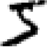

y_train[0]

sgd_clf.fit(X_train[:1000], y_train[:1000])   #y_train, not y_train_5
sgd_clf.predict([some_digit]) #some_digit=X[0]

y_train[0]

############################
Note: the prediction result base on training the SGDClassifier with all training dataset is different with the prediction result base on using first thousand of training set to train the SGDClassifier since the different decision score.
############################
​​​​​That was easy! This code trains the SGDClassifier on the training set using the original target classes from 0 to 9 (y_train), instead of the 5-versus-all target classes (y_train_5). Then it makes a prediction (a correct one in this case). Under the hood,
Scikit-Learn actually trained 10 binary classifiers, got their decision scores for the image, and selected the class with the highest score.

To see that this is indeed the case, you can call the decision_function() method. Instead of returning just one score per instance, it now returns 10 scores, one per class:

some_digit_dicision_scores = sgd_clf.decision_function([some_digit])
some_digit_dicision_scores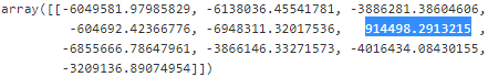

The highest score is indeed the one corresponding to class 5:

np.argmax(some_digit_dicision_scores) #return the index of the maximum value

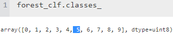
sgd_clf.classes_

sgd_clf.classes_[5] #np.argmax(some_digit_dicision_scores) ==5
#output: the result is a class 5

##################################
WARNING
When a classifier is trained, it stores the list of target classes in its classes_ attribute, ordered by value. In this case, the index of each class in the classes_ array conveniently matches the class itself (e.g., the class at index 5 happens to be class 5), but in general you won’t be so lucky.
##################################
If you want to force ScikitLearn to use one-versus-one or one-versus-all, you can use the OneVsOneClassifier or OneVsRestClassifier classes. Simply create an instance of OneVsOneClassifier or OneVsRestClassifier and pass a binary classifier to its constructor.

For example, this code creates a multiclass classifier using the OvO strategy, based on a SGDClassifier:

from sklearn.multiclass import OneVsOneClassifier

ovo_clf = OneVsOneClassifier(SGDClassifier(random_state=42))
ovo_clf.fit(X_train, y_train)
ovo_clf.predict([some_digit]) #some_digit=X[0]

len(ovo_clf.estimators_) # N*(N–1)/2 = 10*(10-1)/2

one-versus-all (OvA)strategy (also called one-versus-the-rest), base on SVC.

from sklearn.svm import SVC
from sklearn.multiclass import OneVsRestClassifier

ovr_clf = OneVsRestClassifier( SVC(gamma="auto", random_state=42) )
ovr_clf.fit(X_train[:1000], y_train[:1000])
ovr_clf.predict([some_digit])

len(ovr_clf.estimators_)

Training a RandomForestClassifier is just as easy:

#we set n_estimators=100 to be future-proof since this will be the default value in Scikit-Learn 0.22
#forest_clf = RandomForestClassifier(random_state=42, n_estimators=100)
forest_clf.fit(X_train, y_train)
forest_clf.predict([some_digit])

len(forest_clf.estimators_)

This time Scikit-Learn did not have to run OvA or OvO because Random Forest classifiers can directly classify instances into multiple classes. You can call predict_proba() to get the list of probabilities that the classifier assigned to each instance for each class:

forest_clf.predict_proba([some_digit])

You can see that the classifier is fairly confident about its prediction: the 0.9 at the 5th index in the array means that the model estimates an 90% probability that the image represents a 5. It also thinks that the image could instead be a 2 or a 3 (1% chance and 8% chance).

Now of course you want to evaluate these classifiers. As usual, you want to use cross-validation. Let’s evaluate the SGDClassifier’s accuracy using the cross_val_score() function:

cross_val_score(sgd_clf, X_train, y_train, cv=3, scoring="accuracy")

It gets over 85% on all test folds. If you used a random classifier, you would get 10% accuracy(select 1 / 10 digits), so this is not such a bad score, but you can still do much better. For example, simply scaling the inputs increases accuracy above 89%:

from sklearn.preprocessing import StandardScaler

scaler = StandardScaler()
X_train_scaled = scaler.fit_transform(X_train.astype(np.float64))
cross_val_score(sgd_clf, X_train_scaled, y_train, cv=3, scoring="accuracy")

https://blog.csdn.net/Linli522362242/article/details/103387527{Standardization is quite different: first it subtracts the mean value (so standardized values always have a zero mean), and then it divides by the variance so that the resulting distribution has unit variance. }

Error Analysis