


cp3 A Tour of ML Classifiers_stratify_bincount_likelihood_logistic regression_odds ratio_decay_L2
Maximum margin classification with support vector machines
Another powerful and widely used learning algorithm is the Support Vector Machine (SVM), which can be considered an extension of the perceptron. Using the perceptron algorithm, we minimized misclassification errors. However, in SVMs our
optimization objective is to maximize the margin. The margin is defined as the distance between the separating hyperplane (decision boundary) and the training samples that are closest to this hyperplane, which are the so-called support vectors(on support hyperplane).
This is illustrated in the following figure:

Maximum margin intuition
The rationale behind having decision boundaries with large margins is that they tend to have a lower generalization error(for new instances/data) whereas models with small margins are more prone to overfitting. To get an idea of the margin maximization, let's take a closer look at those positive and negative hyperplanes that are parallel to the decision boundary, which can be expressed as follows:![]()
![]()
If we subtract those two linear equations (1) and (2) from each other, we get:![]()
We can normalize this equation by the length of the vector w, which is defined as follows:![]() # m features
# m features
So we arrive at the following equation: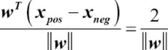
05_Support Vector Machines_hinge_support vectors_decision function_Lagrange multiplier拉格朗日乘数_C~slack_Linli522362242的专栏-CSDN博客 : 05_Support Vector Machines_hinge_support vectors_decision function_Lagrange multiplier
The left side of the preceding equation can then be interpreted as the distance between the positive and negative hyperplane(supporting hyperplanes), which is the so-called margin that we want to maximize.
Now, the objective function of the SVM becomes the maximization of this margin by maximizing ![]() under the constraint that the samples are classified correctly, which can be written as:
under the constraint that the samples are classified correctly, which can be written as:![]()
![]()
![]() Here, N is the number of samples in our dataset.
Here, N is the number of samples in our dataset.
These two equations basically say that all negative samples should fall on one side of the negative hyperplane, whereas all the positive samples should fall behind the positive hyperplane, which can also be written more compactly as follows:![]()
In practice though, it is easier to minimize the reciprocal term ![]() , which can be solved by quadratic programming.
, which can be solved by quadratic programming.
05_Support Vector Machines_02_Polynomial Kernel_Gaussian RBF_Kernelized SVM Regression_Quadratic Programming
05_Support Vector Machines_02_Polynomial Kernel_Gaussian RBF_Kernelized SVM Regression_Quadratic Pro_Linli522362242的专栏-CSDN博客
Dealing with a nonlinearly separable case using slack variables
Although we don't want to dive much deeper into the more involved mathematical concepts behind the maximum-margin classification, let us briefly mention the slack variable ![]() , which was introduced by Vladimir Vapnik in 1995 and led to the socalled soft-margin classification. The motivation for introducing the slack variable
, which was introduced by Vladimir Vapnik in 1995 and led to the socalled soft-margin classification. The motivation for introducing the slack variable ![]() was that the linear constraints need to be relaxed for nonlinearly separable data to allow the convergence of the optimization in the presence of misclassifications, under appropriate cost penalization.
was that the linear constraints need to be relaxed for nonlinearly separable data to allow the convergence of the optimization in the presence of misclassifications, under appropriate cost penalization.
soft margin classification : 05_Support Vector Machines_hinge_support vectors_decision function_Lagrange multiplier拉格朗日乘数_C~slack_Linli522362242的专栏-CSDN博客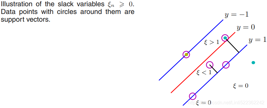
The positive-values slack variable is simply added to the linear constraints:![]()
![]()
So the new objective to be minimized (subject to the preceding constraints) becomes:![]()
Using the variable C(penalty factor), we can then control the penalty for misclassification. Large values of C correspond to large error penalties whereas we are less strict about misclassification errors if we choose smaller values for C. We can then we use the parameter C to control the width of the margin and therefore tune the bias-variance trade-off as illustrated in the following figure: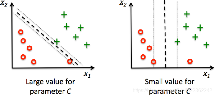
This concept is related to regularization, which we discussed in the previous section in the context of regularized regression where decreasing the value of C increases the bias and lowers the variance of the model.
Now that we have learned the basic concepts behind a linear SVM, let us train an SVM model to classify the different flowers in our Iris dataset:
from matplotlib.colors import ListedColormap
import matplotlib.pyplot as plt


def plot_decision_regions(X, y, classifier, test_idx=None, resolution=0.02):

    # setup marker generator and color map
    markers = ('s', 'x', 'o', '^', 'v')
    colors = ('red', 'blue', 'lightgreen', 'gray', 'cyan')
    cmap = ListedColormap( colors[:len(np.unique(y))] )#########

    # plot the decision surface
    x1_min, x1_max = X[:, 0].min() - 1, X[:, 0].max() + 1 #feature 0
    x2_min, x2_max = X[:, 1].min() - 1, X[:, 1].max() + 1 #feature 1
    # np.arange(x1_min, x1_max, resolution) : feature0 array({min-1, ..., max+1})
    # np.arange(x2_min, x2_max, resolution) : feature1 array({min-1, ..., max+1})

    xx1, xx2 = np.meshgrid(np.arange(x1_min, x1_max, resolution),
                           np.arange(x2_min, x2_max, resolution))
    #xx1, xx2 are both two dimension array with same shape
    #ravel(): Return a contiguous flattened array(one dimension)
            #feature0 array({min-1, ..., max+1,..,min-1, ..., max+1})
            #feature1 array({min-1, ..., max+1,..,min-1, ..., max+1})
    #np.array([xx1.ravel(), xx2.ravel()]): two dimension array(features, samples)
    Z = classifier.predict( np.array([xx1.ravel(), xx2.ravel()]).T )#(samples, features)
    Z = Z.reshape(xx1.shape)

                #axis,axis,height
    plt.contourf(xx1, xx2, Z, alpha=0.3, cmap=cmap)######decision boundaries
    plt.xlim(xx1.min(), xx1.max())
    plt.ylim(xx2.min(), xx2.max())

    for idx, cl in enumerate(np.unique(y)): #cl: class label in dataset X
        plt.scatter(x=X[y == cl, 0], #selection
                    y=X[y == cl, 1],
                    alpha=0.8,
                    c=colors[idx],
                    marker=markers[idx],
                    label=cl,
                    edgecolor='black')

    # highlight test examples
    if test_idx:
        # plot all examples
        X_test, y_test = X[test_idx, :], y[test_idx]

        plt.scatter(X_test[:, 0],
                    X_test[:, 1],
                    c='',
                    edgecolor='black',
                    alpha=1.0,
                    linewidth=1,
                    marker='o',
                    s=100,
                    label='test set')

from sklearn.svm import SVC

svm = SVC(kernel='linear', C=1.0, random_state=1)
svm.fit(X_train_std, y_train)
plot_decision_regions(X_combined_std, y_combined,
                      classifier=svm, test_idx = range(105, 150)
                     )
plt.xlabel('petal length [standarized]')
plt.ylabel('petal width [standarized]')
plt.legend(loc='upper left')
plt.show()
Note
Logistic regression versus support vector machines
In practical classification tasks, linear logistic regression and linear SVMs often yield very similar results. Logistic regression tries to maximize the conditional likelihoods of the training data![]() , which makes it more prone to outliers than SVMs(比支持向量机更易于处理离群点), which mostly care about the points that are closest to the decision boundary (support vectors). On the other hand, logistic regression has the advantage that it is a simpler model and can be implemented more easily. Furthermore, logistic regression models can be easily updated, which is attractive when working with streaming data.
, which makes it more prone to outliers than SVMs(比支持向量机更易于处理离群点), which mostly care about the points that are closest to the decision boundary (support vectors). On the other hand, logistic regression has the advantage that it is a simpler model and can be implemented more easily. Furthermore, logistic regression models can be easily updated, which is attractive when working with streaming data.
Alternative implementations in scikit-learn
The scikit-learn library's Perceptron and LogisticRegression classes, which we used in the previous sections, make use of the LIBLINEAR library, which is a highly optimized C/C++ library developed at the National Taiwan University (http://www.csie.ntu.edu.tw/~cjlin/liblinear/). Similarly, the SVC class that we used to train an SVM makes use of LIBSVM, which is an equivalent C/C++ library specialized for SVMs (http://www.csie.ntu.edu.tw/~cjlin/libsvm/).
The advantage of using LIBLINEAR and LIBSVM over native Python implementations is that they allow the extremely quick training of large amounts of linear classifiers. However, sometimes our datasets are too large to fit into computer memory. Thus, scikit-learn also offers alternative implementations via the SGDClassifier class, which also supports online learning via the partial_fit method. The concept behind the SGDClassifier class is similar to the stochastic gradient algorithm that we implemented in cp2_TrainingSimpleMachineLearningAlgorithmsForClassification_meshgrid_ravel_contourf_OvA_GradientDes_Linli522362242的专栏-CSDN博客
cp02_TrainingSimpleMachineLearningAlgorithmsForClassification_meshgrid_ravel_contourf_OvA_GradientDescent, for Adaline. We could initialize the stochastic gradient descent version of the perceptron, logistic regression, and a support vector machine(uses "hinge" loss, ![]() ==>hinge loss
==>hinge loss 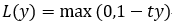 (当t和y的符号相同时(表示y预测正确)并且|y|≥1时,hinge loss为0(since max(0, 1-ty<0);当t和y的符号相反时,hinge loss随着y的增大线性增大, since max(0, 1-ty>0)==>1-ty ~~similart to ~~05_Support Vector Machines_hinge_support vectors_decision function_Lagrange multiplier拉格朗日乘数_C~slack_Linli522362242的专栏-CSDN博客) with default parameters as follows:
from sklearn.linear_model import SGDClassifier

ppn = SGDClassifier( loss="perceptron")
lr = SGDClassifier( loss="log") # logistic regression
svm = SGDClassifier( loss='hinge') # a support vector machine
Solving nonlinear problems using a kernel SVM
Another reason why SVMs enjoy high popularity among machine learning practitioners is that it can be easily kernelized to solve nonlinear classification problems. Before we discuss the main concept behind a kernel SVM, let's first create a sample dataset to see what such a nonlinear classification problem may look like.
Solving nonlinear problems using a kernel SVM

Using the following code, we will create a simple dataset that has the form of an XOR(Exclusive OR d3_10_Introduction to Artificial Neural Network w Keras1_HuberLoss_astype_dtype_DNN_MLP_G.gv.pdf_EMA_Linli522362242的专栏-CSDN博客,相同则0,不同则1) gate using the logical_or function from NumPy, where 100 samples will be assigned the class label 1, and 100 samples will be assigned the class label -1:
import matplotlib.pyplot as plt
import numpy as np

np.random.seed(1)
X_xor = np.random.randn(200, 2)

#label
#XOR 2个input的符号 相同则0 不同则1
y_xor = np.logical_xor( X_xor[:, 0] >0, # -5.28171752e-01
                        X_xor[:, 1] >0) # -1.07296862e+00
#return
# in y_xor(size=200): True(for example: 1.62434536e+00, -6.11756414e-01 )
#                 or False(for example: -5.28171752e-01, -1.07296862e+00)

y_xor = np.where(y_xor, 1, -1)
# in y_xor:  1 or -1

#符号 相同则1: 1.62434536e+00, -6.11756414e-01
plt.scatter(X_xor[y_xor==1, 0],
            X_xor[y_xor==1, 1],
            c='b', marker='x',
            label='1'
           )
#符号 不同则0: -5.28171752e-01, -1.07296862e+00 ==>-1 np.where(y_xor, 1, -1)
plt.scatter(X_xor[y_xor==-1,0],
            X_xor[y_xor==-1,1],
            c='r', marker='s',
            label='-1')

plt.xlim([-3,3])
plt.ylim([-3,3])
plt.legend(loc='best')
plt.show()
After executing the code, we will have an XOR dataset with random noise, as shown in the following figure:

Obviously, we would not be able to separate samples from the positive and negative class very well using a linear hyperplane as a decision boundary via the linear logistic regression or linear SVM model that we discussed in earlier sections.
The basic idea behind kernel methods to deal with such linearly inseparable data is to create nonlinear combinations of the original features to project them onto a higher-dimensional space via a mapping function![]() where it becomes linearly separable. As shown in the following figure, we can transform a two-dimensional dataset onto a new three-dimensional feature space where the classes become separable via the following projection:
where it becomes linearly separable. As shown in the following figure, we can transform a two-dimensional dataset onto a new three-dimensional feature space where the classes become separable via the following projection:![]()
This allows us to separate the two classes shown in the plot via a linear hyperplane that becomes a nonlinear decision boundary if we project it back onto the original feature space:
Kernelized SVM![]() : https://blog.csdn.net/Linli522362242/article/details/104280075
: https://blog.csdn.net/Linli522362242/article/details/104280075
Lagrange multiplier minimize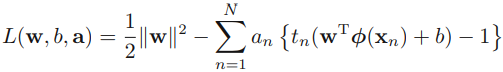 ==> dual representation maximize
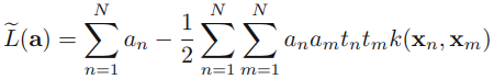 OR
OR 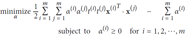 ==>
==> : 05_Support Vector Machines_hinge_support vectors_decision function_Lagrange multiplier拉格朗日乘数_C~slack_Linli522362242的专栏-CSDN博客
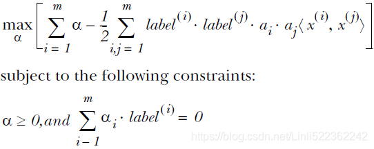
The hard margin(without slacks variables): 05_Support Vector Machines_02_Polynomial Kernel_Gaussian RBF_Kernelized SVM Regression_Quadratic Pro_Linli522362242的专栏-CSDN博客

Quadratic Programming  ==>
==> : 05_Support Vector Machines_02_Polynomial Kernel_Gaussian RBF_Kernelized SVM Regression_Quadratic Pro_Linli522362242的专栏-CSDN博客
Using the kernel trick to find separating hyperplanes in high-dimensional space
To solve a nonlinear problem using an SVM, we would transform the training data onto a higher-dimensional feature space via a mapping function![]() and train a linear SVM model to classify the data in this new feature space. Then, we can use the same mapping function
and train a linear SVM model to classify the data in this new feature space. Then, we can use the same mapping function![]() to transform new, unseen data to classify it using the linear SVM model.
to transform new, unseen data to classify it using the linear SVM model.
However, one problem with this mapping approach is that the construction of the new features is computationally very expensive, especially if we are dealing with high-dimensional data. This is where the so-called kernel trick comes into
play. Although we didn't go into much detail about how to solve the quadratic programming (05_Support Vector Machines_02_Polynomial Kernel_Gaussian RBF_Kernelized SVM Regression_Quadratic Programming: 05_Support Vector Machines_02_Polynomial Kernel_Gaussian RBF_Kernelized SVM Regression_Quadratic Pro_Linli522362242的专栏-CSDN博客) task to train an SVM, in practice all we need is to replace the dot product ![]() by
by ![]() . In order to save the expensive step of calculating
. In order to save the expensive step of calculating
this dot product between two points explicitly, we define a so-called kernel function:![]() .
.
One of the most widely used kernels is the Radial Basis Function (RBF) kernel or simply called the Gaussian kernel: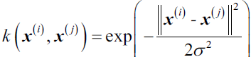
This is often simplified to: ![]()
Here, ![]() is a free parameter that is to be optimized. 05_Support Vector Machines_02_Polynomial Kernel_Gaussian RBF_Kernelized SVM Regression_Quadratic Pro_Linli522362242的专栏-CSDN博客
is a free parameter that is to be optimized. 05_Support Vector Machines_02_Polynomial Kernel_Gaussian RBF_Kernelized SVM Regression_Quadratic Pro_Linli522362242的专栏-CSDN博客

Figure 5-8. Similarity features using the Gaussian RBF
summary: assuming you drop the original features
dataset ==>Two k(dataset_X, landmark_X' from dataset_X)= ==>new dataset(exponential value, exponential value ) which is linearly separable.
Roughly speaking, the term kernel can be interpreted as a similarity function between a pair of samples. The minus sign inverts the distance measure into a similarity score and, due to the exponential term, the resulting similarity score will fall into a range between 1 (for exactly similar samples) and 0 (for very dissimilar samples).
Now that we defined the big picture behind the kernel trick, let us see if we can train a kernel SVM that is able to draw a nonlinear decision boundary that separates the XOR data well. Here, we simply use the SVC class from scikit-learn that we imported earlier and replace the kernel='linear' parameter with kernel='rbf':
svm = SVC(kernel='rbf', random_state=1, gamma=0.10, C=10.0)
svm.fit(X_xor, y_xor)
#figsize:  defaults to rcParams["figure.figsize"] = [6.4, 4.8].
plot_decision_regions(X_xor, y_xor, classifier=svm)
plt.legend(loc='upper left')
plt.tight_layout()
plt.show()
As we can see in the resulting plot, the kernel SVM separates the XOR data relatively well:
The ![]() parameter, which we set to gamma=0.1, can be understood as a cut-off parameter for the Gaussian sphere. If we increase the value for
parameter, which we set to gamma=0.1, can be understood as a cut-off parameter for the Gaussian sphere. If we increase the value for ![]() , we increase the influence or reach of the training samples, which leads to a tighter and bumpier decision boundary.
, we increase the influence or reach of the training samples, which leads to a tighter and bumpier decision boundary.
svm = SVC(kernel='rbf', random_state=1, gamma=0.5, C=10.0)
svm.fit(X_xor, y_xor)
#figsize:  defaults to rcParams["figure.figsize"] = [6.4, 4.8].
plot_decision_regions(X_xor, y_xor, classifier=svm)
plt.legend(loc='upper left')
plt.tight_layout()
plt.show()
To get a better intuition for ![]() , let us apply an RBF kernel SVM to our Iris flower dataset:
, let us apply an RBF kernel SVM to our Iris flower dataset:
# X_combined_std = np.vstack((X_train_std, X_test_std))
# y_combined = np.hstack((y_train, y_test))
svm = SVC( kernel='rbf', random_state=1, gamma=0.2, C=1.0)
svm.fit(X_train_std, y_train)
plot_decision_regions(X_combined_std, y_combined, classifier=svm,
                      test_idx=range(105,150))
plt.xlabel('petal length [standardized]')
plt.ylabel('petal width [standardized]')
plt.legend(loc='upper left')
plt.show()
Since we chose a relatively small value for ![]() , the resulting decision boundary of the RBF kernel SVM model will be relatively soft, as shown in the following figure:
, the resulting decision boundary of the RBF kernel SVM model will be relatively soft, as shown in the following figure:
Now, let us increase the value of ![]() and observe the effect on the decision boundary:
and observe the effect on the decision boundary:
# X_combined_std = np.vstack((X_train_std, X_test_std))
# y_combined = np.hstack((y_train, y_test))
svm = SVC( kernel='rbf', random_state=1, gamma=100, C=1.0)
svm.fit(X_train_std, y_train)
plot_decision_regions(X_combined_std, y_combined, classifier=svm,
                      test_idx=range(105,150))
plt.xlabel('petal length [standardized]')
plt.ylabel('petal width [standardized]')
plt.legend(loc='upper left')
plt.show()
In the resulting plot, we can now see that the decision boundary around the classes 0 and 1 is much tighter using a relatively large value of ![]() :
:

Although the model fits the training dataset very well, such a classifier will likely have a high generalization error on unseen data. This illustrates that the ![]() parameter also plays an important role in controlling overfitting.
parameter also plays an important role in controlling overfitting.
Decision tree learning
Decision tree classifiers are attractive models if we care about interpretability. As the name decision tree suggests, we can think of this model as breaking down our data by making decision based on asking a series of questions.
Let's consider the following example in which we use a decision tree to decide upon an activity on a particular day:
Based on the features in our training set, the decision tree model learns a series of questions to infer the class labels of the samples. Although the preceding figure illustrates the concept of a decision tree based on categorical variables, the same
concept applies if our features are real numbers, like in the Iris dataset. For example, we could simply define a cut-off value along the sepal width feature axis and ask a binary question "Is sepal width ≥ 2.8 cm?."
Using the decision algorithm, we start at the tree root and split the data on the feature that results in the largest information gain (IG), which will be explained in more detail in the following section. In an iterative process, we can then repeat this splitting procedure at each child node until the leaves are pure. This means that the samples at each node all belong to the same class. In practice, this can result in a very deep tree with many nodes, which can easily lead to overfitting. Thus, we typically want to prune the tree by setting a limit for the maximal depth of the tree.
Maximizing information gain – getting the most bang for your buck
In order to split the nodes at the most informative features, we need to define an objective function that we want to optimize via the tree learning algorithm. Here, our objective function is to maximize the information gain at each split, which we define as follows:![]()
Here, f is the feature to perform the split, ![]() and
and ![]() are the dataset of the parent and jth child node, I is our impurity measure,
are the dataset of the parent and jth child node, I is our impurity measure, ![]() is the total number of samples at the parent node, and
is the total number of samples at the parent node, and ![]() is the number of samples in the jth child node. As we can see, the information gain is simply the difference between the impurity of the parent node and the sum of the child node impurities—the lower the impurity of the child nodes, the larger the information gain.
is the number of samples in the jth child node. As we can see, the information gain is simply the difference between the impurity of the parent node and the sum of the child node impurities—the lower the impurity of the child nodes, the larger the information gain.
However, for simplicity and to reduce the combinatorial search space, most libraries (including scikit-learn) implement binary decision trees. This means that each parent node is split into two child nodes, ![]() and
and ![]() :
:
information gain: 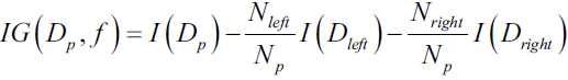
Now, the three impurity measures or splitting criteria that are commonly used in binary decision trees are Gini impurity ( ![]() ), entropy (
), entropy ( ![]() ), and the classification error (
), and the classification error ( ![]() ). Let's start with the definition of entropy for all non-empty classes
). Let's start with the definition of entropy for all non-empty classes ![]() :
:
(cross)entropy:  0 ≤
0 ≤  ≤ 1
≤ 1
Here, ![]() is the proportion of the samples that belongs to class i for a particular node t. The entropy is therefore 0 if all samples at a node belong to the same class, and the entropy is maximal if we have a uniform class distribution. For example, in a binary class setting, the entropy is 0(= -(1*0 + 0*
is the proportion of the samples that belongs to class i for a particular node t. The entropy is therefore 0 if all samples at a node belong to the same class, and the entropy is maximal if we have a uniform class distribution. For example, in a binary class setting, the entropy is 0(= -(1*0 + 0*![]() (0)) ) if p (i =1| t ) =1 or p(i = 0 | t ) = 0. If the classes are distributed uniformly with p (i =1| t ) = 0.5 and p(i = 0 | t ) = 0.5, the entropy is 1(= - (0.5*-1 + 0.5*-1) ) . Therefore, we can say that the entropy criterion attempts to maximize the mutual information in the tree.
(0)) ) if p (i =1| t ) =1 or p(i = 0 | t ) = 0. If the classes are distributed uniformly with p (i =1| t ) = 0.5 and p(i = 0 | t ) = 0.5, the entropy is 1(= - (0.5*-1 + 0.5*-1) ) . Therefore, we can say that the entropy criterion attempts to maximize the mutual information in the tree.
Intuitively, the Gini impurity can be understood as a criterion to minimize the probability of misclassification:
Gini impurity(Gini index): 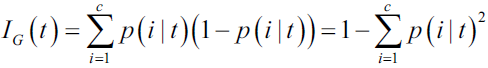 0 ≤ ≤ 1
 0 ≤ ˆpmk ≤ 1
04_TrainingModels_04_gradient decent with early stopping for softmax regression_ entropy_Gini:
04_TrainingModels_04_gradient decent with early stopping for softmax regression_ entropy_Gini_Linli522362242的专栏-CSDN博客
the Gini index takes on a small value if all of the ˆpmk’s (OR ![]() ) are close to zero or one. For this reason the Gini index is referred to as a measure of node purity—a small value indicates that a node contains predominantly显著地 observations(or samples) from a single class.(eg, K=2, means the mth node is relatively pure, p=0.9, p *q= 0.9*0.1== 0.09, Gini index at mth node=0.9*0.1+0.1*0.9=0.18 )
) are close to zero or one. For this reason the Gini index is referred to as a measure of node purity—a small value indicates that a node contains predominantly显著地 observations(or samples) from a single class.(eg, K=2, means the mth node is relatively pure, p=0.9, p *q= 0.9*0.1== 0.09, Gini index at mth node=0.9*0.1+0.1*0.9=0.18 )
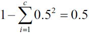
Similar to entropy, the Gini impurity is maximal if the classes are perfectly mixed(distributed uniformly), for example, in a binary class setting ( ![]() ):
): 
However, in practice both the Gini impurity and entropy typically yield very similar results and it is often not worth spending much time on evaluating trees using different impurity criteria rather than experimenting with different pruning cut-offs.
Another impurity measure is the classification error: ![]()
This is a useful criterion for pruning but not recommended for growing a decision tree, since it is less sensitive to changes in the class probabilities of the nodes. We can illustrate this by looking at the two possible splitting scenarios shown in the following figure:
We start with a dataset ![]() at the parent node
at the parent node ![]() that consists of 40 samples from class 1 and 40 samples from class 2 that we split into two datasets
that consists of 40 samples from class 1 and 40 samples from class 2 that we split into two datasets ![]() and
and ![]() , respectively.
, respectively.
The information gain using the classification error ![]() as a splitting criterion would be the same (
as a splitting criterion would be the same ( ![]() ) in both scenario A and B:
) in both scenario A and B:

#########################
However, the Gini impurity would favor the split in scenario A(![]() ) over scenario B(
) over scenario B( ![]() ), which is indeed more pure:
), which is indeed more pure:

https://blog.csdn.net/Linli522362242/article/details/104542381
example: 
![]() and 1 ==
and 1 == ![]() +
+ ![]() +
+ ![]() (the sum of all probabilities of all classes is equal to 1)
(the sum of all probabilities of all classes is equal to 1)
#########################
Similarly, the entropy criterion would favor scenario B( ![]() ) over scenario A(
) over scenario A(![]() ) :
) :

https://blog.csdn.net/Linli522362242/article/details/104542381
the entropy of the ith node. For example, the depth-2 left node in Figure 6-1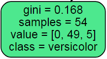 has an entropy equal to
 ![]() .
.
So should you use Gini impurity or entropy? The truth is, most of the time it does not make a big difference: they lead to similar trees. Gini impurity is slightly faster to compute, so it is a good default. However, when they differ, Gini impurity tends to isolate the most frequent class in its own branch of the tree, while entropy tends to produce slightly more balanced trees.
For a more visual comparison of the three different impurity criteria that we discussed previously, let us plot the impurity indices for the probability range [0, 1] for class 1. Note that we will also add a scaled version of the entropy (entropy / 2) to
observe that the Gini impurity is an intermediate measure between entropy and the classification error. The code is as follows:
import matplotlib.pyplot as plt
import numpy as np

def gini(p):
    return p*(1-p) + (1-p)*( 1-(1-p) )

def entropy(p):
    return -p*np.log2(p) -(1-p)*np.log2(1-p)

def error(p):
    return 1- np.max([p, 1-p])

x = np.arange(0.0, 1.0, 0.01)

ent = [entropy(p) if p!=0 else None
       for p in x]
# a scaled version of the entropy (entropy / 2)
sc_ent = [e*0.5 if e else None
          for e in ent]

err = [error(i) for i in x]
#ge = [ gini(i) for i in x ]##OR

fig = plt.figure()
ax = plt.subplot(111)                 #gini(x) is a simple operation
for i, lab, ls, c in zip([ent, sc_ent, gini(x), err],
                         ['Entropy', "Entropy (scaled)",
                          'Gini impurity',
                          'Misclassification error'],
                         ['-', '-', '--', '-.'],
                         ['black', 'lightgray', 'red', 'green', 'blue']
                        ):
    line = ax.plot(x, i, label=lab, linestyle=ls, lw=2, color=c)
#bbox_to_anchor: https://blog.csdn.net/chichoxian/article/details/101058046
ax.legend(loc='upper center', bbox_to_anchor=(0.5, 1.2),######
          ncol=3, fancybox=True, shadow=True)
ax.axhline(y=0.5, linewidth=1, color='k', linestyle='--')
ax.axhline(y=1, linewidth=1, color='k', linestyle='--')
plt.ylim([0, 1.1])
plt.xlabel('p(i=1)')
plt.ylabel('impurity index')
plt.show()
The plot produced by the preceding code example is as follows:

Building a decision tree
Decision trees can build complex decision boundaries by dividing the feature space into rectangles. However, we have to be careful since the deeper the decision tree, the more complex the decision boundary becomes, which can easily result in
overfitting.
Using scikit-learn, we will now train a decision tree with a maximum depth of 4, using gini as a criterion for impurity(Gini impurity tends to isolate the most frequent class in its own branch of the tree). Although feature scaling may be desired for visualization purposes, note that feature scaling is not a requirement for decision tree algorithms. The code is as follows:
from sklearn.tree import DecisionTreeClassifier

tree_model = DecisionTreeClassifier(criterion="gini",
                                    max_depth=4,###########
                                    random_state=1)
tree_model.fit(X_train, y_train)

X_combined = np.vstack((X_train, X_test))
y_combined = np.hstack((y_train, y_test))
plot_decision_regions(X_combined, y_combined,
                      classifier=tree_model,
                      test_idx=range(105,150))
plt.xlabel('petal length [cm]')
plt.ylabel('petal width [cm]')
plt.legend(loc='upper left')
plt.tight_layout()
plt.show()
After executing the code example, we get the typical axis-parallel decision boundaries of the decision tree:

A nice feature in scikit-learn is that it allows us to export the decision tree as a .dot file after training, which we can visualize using the GraphViz program, for example.
This program is freely available from http://www.graphviz.org and supported by Linux, Windows, and macOS. In addition to GraphViz, we will use a Python library called pydotplus, which has capabilities similar to GraphViz and allows us to convert .dot data files into a decision tree image file. After you installed GraphViz (by following the instructions on http://www.graphviz.org/Download.php), you can install pydotplus directly via the pip installer, for example, by executing the following command in your Terminal:
>activate tensorflow
> pip install pydotplus
Note
Note that on some systems, you may have to install the pydotplus prerequisites manually by executing the following commands:
pip3 install graphviz # https://blog.csdn.net/Linli522362242/article/details/104542381
pip3 install pyparsing
06_Decision Trees_01_graphviz_Gini_Entropy_Decision Tree_CART_prune_Regression_Classification_Tree
https://blog.csdn.net/Linli522362242/article/details/104542381
The following code will create an image of our decision tree in PNG format in our local directory:
from sklearn.tree import export_graphviz
from graphviz import Source
import os
os.environ['PATH'] += os.pathsep + "C:/Graphviz2.38/bin"# " directory" where you intall graphviz

dot_data = export_graphviz(
    tree_model,
    rounded=True,
    filled=True,
    #OR iris.target_names
    #   array(['setosa', 'versicolor', 'virginica'], dtype='<U10')
    #class_names = iris.target_names
    class_names = ['Setosa', 'Versicolor', 'Virginica'],
    #OR feature_names=['petal length', 'petal width'],
    feature_names = iris.feature_names[2:],
    out_file = os.path.join('iris_tree.dot'),
)
Source.from_file('iris_tree.dot')

from sklearn.tree import export_graphviz
# from graphviz import Source
# import os
# os.environ['PATH'] += os.pathsep + "C:/Graphviz2.38/bin"# " directory" where you intall graphviz
from pydotplus import graph_from_dot_data

dot_data = export_graphviz(
    tree_model,
    rounded=True,
    filled=True,
    #OR iris.target_names
    #   array(['setosa', 'versicolor', 'virginica'], dtype='<U10')
    #class_names = iris.target_names
    class_names = ['Setosa', 'Versicolor', 'Virginica'],
    #OR feature_names=['petal length', 'petal width'],
    feature_names = iris.feature_names[2:],
    out_file = None,##############
)
# Source.from_file('iris_tree.dot')
graph = graph_from_dot_data(dot_data)
graph.write_png('tree.png')![]()
from IPython.display import Image
Image(filename='tree.png', width=600)
By using the out_file=None setting, we directly assigned the dot data to a dot_data variable, instead of writing an intermediate tree.dot file to disk. The arguments for filled, rounded, class_names, and feature_names are optional but make the resulting image file visually more appealing by adding color, rounding the box edges, showing the name of the majority class label at each node, and displaying the feature names in the splitting criterion. These settings resulted in the following decision tree image:
Looking at the decision tree figure, we can now nicely trace back the splits that the decision tree determined from our training dataset. We started with 105 samples at the root and split them into two child nodes with 35 and 70 samples, using the petal
width cut-off ≤ 0.75 cm. After the first split, we can see that the left child node is already pure and only contains samples from the Iris-setosa class (Gini Impurity =0). The further splits on the right are then used to separate the samples from the Iris-versicolor and Iris-virginica class.
Looking at this tree, and the decision region plot of the tree, we see that the decision tree does a very good job of separating the flower classes. Unfortunately, scikit-learn currently does not implement functionality to manually post-prune a decision tree. However, we could go back to our previous code example, change the max_depth of our decision tree to 3, and compare it to our current model, but we leave this as an exercise for the interested reader.
from sklearn.tree import DecisionTreeClassifier

tree_model = DecisionTreeClassifier(criterion="gini",
                                    max_depth=3,###########
                                    random_state=1)
tree_model.fit(X_train, y_train)

X_combined = np.vstack((X_train, X_test))
y_combined = np.hstack((y_train, y_test))
plot_decision_regions(X_combined, y_combined,
                      classifier=tree_model,
                      test_idx=range(105,150))
plt.xlabel('petal length [cm]')
plt.ylabel('petal width [cm]')
plt.legend(loc='upper left')
plt.tight_layout()
plt.show()
from sklearn.tree import export_graphviz
# from graphviz import Source
# import os
# os.environ['PATH'] += os.pathsep + "C:/Graphviz2.38/bin"# " directory" where you intall graphviz
from pydotplus import graph_from_dot_data

dot_data = export_graphviz(
    tree_model,
    rounded=True,
    filled=True,
    #OR iris.target_names
    #   array(['setosa', 'versicolor', 'virginica'], dtype='<U10')
    #class_names = iris.target_names
    class_names = ['Setosa', 'Versicolor', 'Virginica'],
    #OR feature_names=['petal length', 'petal width'],
    feature_names = iris.feature_names[2:],
    out_file = None,##############
)
# Source.from_file('iris_tree.dot')
graph = graph_from_dot_data(dot_data)
graph.write_png('tree.png')

from IPython.display import Image
Image(filename='tree.png', width=600)
Combining multiple decision trees via random forests
cp3 A Tour of ML Classifiers_3_ random forests_knn_Linli522362242的专栏-CSDN博客


 9183
9183


 被折叠的 条评论
为什么被折叠?
被折叠的 条评论
为什么被折叠?
 到【灌水乐园】发言


