


cp13_Parallelizing NN Training w TF_printoptions(precision)_squeeze_shuffle_batch_repeat_image process_map_celeba_tfrecord
https://blog.csdn.net/Linli522362242/article/details/112386820
13_Loading & Prep 4_[..., np.newaxis]_ExitStack_walk_file操作_timeit_正则_feature vector embed_Text Toke_read & write tfrecord files
https://blog.csdn.net/Linli522362242/article/details/108108665
This was all we needed to do to fetch and use the CelebA image dataset.
Next, we will proceed with the second approach for fetching a dataset from tensorflow_datasets. There is a wrapper function called load() that combines the three steps for fetching a dataset in one. Let's see how it can be used to fetch the MNIST digit dataset:
mnist, mnist_info = tfds.load('mnist', with_info=True,
                               shuffle_files=False)
print( mnist_info )
print( mnist.keys() )![]()
As we can see, the MNIST dataset is split into two partitions. Now, we can take the train partition, apply a transformation to convert the elements from a dictionary to
a tuple, and visualize 10 examples:
ds_train = mnist['train']
assert isinstance( ds_train, tf.data.Dataset )
# ds_train.take(1)
# <TakeDataset shapes: {image: (28, 28, 1), label: ()}, types: {image: tf.uint8, label: tf.int64}>

ds_train = ds_train.map( lambda item: (item['image'], item['label'] )
                       )
# ds_train
# <MapDataset shapes: ((28, 28, 1), ()), types: (tf.uint8, tf.int64)>

ds_train = ds_train.batch(10) #batch size=10 items
batch = next( iter(ds_train) )
print(batch[0].shape, batch[1])# column_0, column_1
# (10, 28, 28, 1) tf.Tensor([4 1 0 7 8 1 2 7 1 6], shape=(10,), dtype=int64)

fig = plt.figure( figsize=(15,6) )
for i, (image, label) in enumerate( zip(batch[0], batch[1]) ):
    ax = fig.add_subplot(2, 5, i+1)
    ax.set_xticks([])
    ax.set_yticks([])
    ax.imshow( image[:, :, 0], cmap='gray_r' )
    ax.set_title( '{}'.format(label), size=15 )

plt.show()
The retrieved example handwritten digits from this dataset are shown as follows:

This concludes our coverage of building and manipulating datasets and fetching datasets from the tensorflow_datasets library. Next, we will see how to build NN models in TensorFlow.
#############################################################
TensorFlow style guide
Note that the official TensorFlow style guide (https://www.tensorflow.org/community/contribute/code_style) recommends using two-character spacing for code indents. However, this book uses four characters for indents as it is more consistent with the official Python style guide and also helps with displaying the code syntax highlighting in many text editors
correctly, as well as the accompanying Jupyter code notebooks at https://github.com/rasbt/python-machinelearning-book-3rd-edition.
#############################################################
Building an NN model in TensorFlow
So far in this chapter, you have learned about the basic utility components of TensorFlow for manipulating tensors and organizing data into formats that we can iterate over during training. In this section, we will finally implement our first predictive model in TensorFlow. As TensorFlow is a bit more flexible but also more complex than machine learning libraries such as scikit-learn, we will start with a simple linear regression model.
The TensorFlow Keras API (tf.keras)
Keras is a high-level NN API and was originally developed to run on top of other libraries such as TensorFlow and Theano. Keras provides a user-friendly and modular programming interface that allows easy prototyping and the building of complex models in just a few lines of code. Keras can be installed independently from PyPI and then configured to use TensorFlow as its backend engine. Keras is tightly integrated into TensorFlow and its modules are accessible through tf.keras. In TensorFlow 2.0, tf.keras has become the primary and recommended approach for implementing models. This has the advantage that it supports TensorFlowspecific functionalities, such as dataset pipelines using tf.data, which you learned about in the previous section. In this book, we will use the tf.keras module to build NN models.
As you will see in the following subsections, the Keras API (tf.keras) makes building an NN model extremely easy. The most commonly used approach for building an NN in TensorFlow is through tf.keras.Sequential(), which allows stacking layers to form a network. A stack of layers can be given in a Python list to a model defined as tf.keras.Sequential(). Alternatively, the layers can be added one by one using the .add() method.
Furthermore, tf.keras allows us to define a model by subclassing tf.keras.Model. This gives us more control over the forward pass by defining the call() method for our model class to specify the forward pass explicitly. We will see examples of both of these approaches for building an NN model using the tf.keras API.
Finally, as you will see in the following subsections, models built using the tf.keras API can be compiled and trained via the .compile() and .fit() methods.
Building a linear regression model
In this subsection, we will build a simple model to solve a linear regression problem.
First, let's create a toy dataset in NumPy and visualize it:
import tensorflow as tf
import numpy as np
import matplotlib.pyplot as plt
%matplotlib inline
#https://www.cnblogs.com/chester-cs/p/11825282.html
X_train = np.arange(10).reshape( (10,1) )
y_train = np.array([1.0, 1.3, 3.1,
2.0, 5.0, 6.3,
6.6, 7.4, 8.0,
9.0])
plt.plot( X_train, y_train, 'o', markersize=10 )
plt.xlabel('x')
plt.ylabel('y')
plt.show()As a result, the training examples will be shown in a scatterplot as follows:
Next, we will standardize the features (mean centering and dividing by the standard deviation) and create a TensorFlow Dataset:
X_train_norm = ( X_train - np.mean(X_train) )/np.std(X_train)

ds_train_orig = tf.data.Dataset.from_tensor_slices(
    ( tf.cast( X_train_norm, tf.float32 ),
      tf.cast( y_train, tf.float32 ) )
)
ds_train_orig![]()
Now, we can define our model for linear regression as 𝑧 = 𝑤x + 𝑏 . Here, we are going to use the Keras API. tf.keras provides predefined layers for building complex NN models, but to start, you will learn how to define a model from scratch. Later in this chapter, you will see how to use those predefined layers.
For this regression problem, we will define a new class derived from the tf.keras.Model class. Subclassing tf.keras.Model allows us to use the Keras tools for exploring a model, training, and evaluation. In the constructor of our class, we will define the parameters of our model, w and b, which correspond to the weight and the bias parameters, respectively. Finally, we will define the call() method to determine how this model uses the input data to generate its output:
class MyModel( tf.keras.Model ):
    def __init__(self):
        super( MyModel, self ).__init__()
        self.w = tf.Variable( 0.0, name='weight' )
        self.b = tf.Variable( 0.0, name='bias' )

    def call(self, x):
        return self.w*x + self.b

model = MyModel()
model.build( input_shape=(None, 1) )
model.summary()
Next, we will instantiate a new model from the MyModel() class that we can train based on the training data. The TensorFlow Keras API provides a method named .summary() for models that are instantiated from tf.keras.Model, which allows us to get a summary of the model components layer by layer and the number of parameters in each layer. Since we have sub-classed our model from tf.keras.Model, the .summary() method is also available to us. But, in order to be able to call model.summary(), we first need to specify the dimensionality of the input (the number of features) to this model. We can do this by calling model.build() with the expected shape of the input data(here is 1):
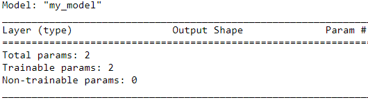
Note that we used None as a placeholder for the first dimension of the expected input tensor via model.build(), which allows us to use an arbitrary batch size. However, the number of features is fixed (here 1) as it directly corresponds to the number of weight parameters of the model. Building model layers and parameters after instantiation by calling the .build() method is called late variable creation. For this simple model, we already created the model parameters in the constructor; therefore, specifying the input_shape via build() has no further effect on our parameters, but still it is needed if we want to call model.summary().
After defining the model, we can define the cost function that we want to minimize to find the optimal model weights. Here, we will choose the mean squared error (MSE) as our cost function. Furthermore, to learn the weight parameters of the model, we will use stochastic gradient descent. In this subsection, we will implement this training via the stochastic gradient descent procedure by ourselves, but in the next subsection, we will use the Keras methods compile() and fit() to do the same thing.
To implement the stochastic gradient descent algorithm, we need to compute the gradients. Rather than manually computing the gradients, we will use the TensorFlow API tf.GradientTape. We will cover tf.GradientTape and its different behaviors in Chapter 14, Going Deeper – The Mechanics of TensorFlow. The code is as follows:
############################
You will find all the basic math operations you need (tf.add(), tf.multiply(), tf.square(), tf.exp(), tf.sqrt(), etc.) and most operations that you can find in NumPy (e.g., tf.reshape(), tf.squeeze(), tf.tile()). Some functions have a different name than in NumPy; for instance, tf.reduce_mean(), tf.reduce_sum(), tf.reduce_max(), and tf.math.log() are the equivalent of np.mean(), np.sum(), np.max() and np.log(). When the name differs, there is often a good reason for it. For example, in TensorFlow you must write tf.transpose(t); you cannot just write t.T like in NumPy. The reason is that the tf.transpose() function does not do exactly the same thing as NumPy’s T attribute: in TensorFlow, a new tensor is created with its own copy of the transposed data, while in NumPy, t.T is just a transposed view on the same data. Similarly, the tf.reduce_sum() operation is named this way because its GPU kernel (i.e., GPU implementation) uses a reduce algorithm that does not guarantee the order in which the elements are added: because 32-bit floats have limited precision, the result may change ever so slightly every time you call this operation. The same is true of tf.reduce_mean() (but of course tf.reduce_max() is deterministic).
tf.math.reduce_mean(
    input_tensor, axis=None, keepdims=False, name=None
)
Reduces input_tensor along the dimensions given in axis by computing the mean of elements across the dimensions in axis. Unless keepdims is true, the rank of the tensor is reduced by 1 for each of the entries in axis, which must be unique. If keepdims is true, the reduced dimensions are retained with length 1.
If axis is None, all dimensions are reduced, and a tensor with a single element is returned.
###########################
https://blog.csdn.net/Linli522362242/article/details/106290394
cost function : ![]()
def loss_fn(y_true, y_pred):
    return tf.reduce_mean( tf.square(y_true-y_pred) )# 1/n*(y-y_pred)**2

## testing the function:
yt = tf.convert_to_tensor([1.0])
yp = tf.convert_to_tensor([1.5])
loss_fn(yt, yp)![]()
###########################
tf.GradientTape(
    persistent=False, watch_accessed_variables=True
)
Record operations for automatic differentiation.
Operations are recorded if they are executed within this context manager and at least one of their inputs is being "watched".
Trainable variables (created by tf.Variable or tf.compat.v1.get_variable, where trainable=True is default in both cases) are automatically watched. Tensors can be manually watched by invoking the watch method on this context manager.
12 _Custom Models and Training with TensorFlow_2_progress_status_bar_Training Loops_concrete : https://blog.csdn.net/Linli522362242/article/details/107459161
###########################
stochastic gradient descent (SGD, update the weights incrementally for each training sample: ![]() (m==1 and added the term
(m==1 and added the term ![]() to the calculation process.) To obtain satisfying results via stochastic gradient descent, it is important to present it training data in a random order; also, we want to shuffle the training set for every epoch to prevent cycleshttps://blog.csdn.net/Linli522362242/article/details/111940633cp12_implement a M ArtificialNN_gzip_mnist_struct_savez_compressed_fetch_openml_back propagation_weight update_L2_Gradient Descent.
to the calculation process.) To obtain satisfying results via stochastic gradient descent, it is important to present it training data in a random order; also, we want to shuffle the training set for every epoch to prevent cycleshttps://blog.csdn.net/Linli522362242/article/details/111940633cp12_implement a M ArtificialNN_gzip_mnist_struct_savez_compressed_fetch_openml_back propagation_weight update_L2_Gradient Descent.
https://blog.csdn.net/Linli522362242/article/details/106290394 09_Up and Running with TensorFlow_2_Autodiff_momentum optimizer_Mini-batchGradientDescent_SavingMode
cost function : ![]()
Equation 4-5. Partial derivatives of the cost function(start with ![]() or i >=1)
or i >=1) ==
==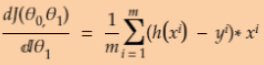 * 2 (without adding the term
 ![]() to the calculation process.)
to the calculation process.)
quation 4-6. Gradient vector of the cost function (![]() for equation 4-5)
for equation 4-5) Note (about derivative_MSE/ derivative_bias term):
  ==
== ![]() *2 (without adding the term
*2 (without adding the term ![]() to the calculation process. AND x_0=1)
to the calculation process. AND x_0=1)
Equation 4-7. Gradient Descent step ![]()
def train(model, inputs, outputs, learning_rate):
    # Since the mean_squared_error() function returns one loss per instance, (if you wanted to
    # apply different weights to each instance, this is where you would do it).
    with tf.GradientTape() as tape:
        current_loss = loss_fn( model(inputs), outputs ) # model = MyModel() # self.w*x + self.b
    # self.w = tf.Variable( 0.0, name='weight' ), self.b = tf.Variable( 0.0, name='bias' )
    # https://blog.csdn.net/Linli522362242/article/details/96429442
    # Next, we ask the tape to compute the gradient of the loss with regard to each
    # trainable variable (not all variables!)
    dW, db = tape.gradient( current_loss,
                            [model.w, model.b] ) #delta_w =derivative_MSE/dw= 2/m *X.T.dot(y-y_pred), delta_b=2/m *(y-y_pred).sum() # both without *1/2
    model.w.assign_sub( learning_rate*dW ) # Subtracts a value from this variable(model.w)
    model.b.assign_sub( learning_rate*db ) # Subtracts a value from this variable(model.b)
Now, we can set the hyperparameters and train the model for 200 epochs. We will create a batched version of the dataset and repeat the dataset with count=None, which will result in an infinitely repeated dataset( but if i>= steps_per_epoch*num_epochs, the for loop will be stopped):
tf.random.set_seed(1)

num_epochs = 200
log_steps = 100
learning_rate = 0.001
batch_size = 1
steps_per_epoch = int( np.ceil( len(y_train)/batch_size ) )#use the whole dataset per epoch

# X_train_norm = ( X_train - np.mean(X_train) )/np.std(X_train)

# ds_train_orig = tf.data.Dataset.from_tensor_slices(
#     ( tf.cast( X_train_norm, tf.float32 ),
#       tf.cast( y_train, tf.float32 ) )
# )
# The .shuffle() method requires an argument called buffer_size,
# # which determines how many elements in the dataset are grouped together before shuffling.
# The elements in the buffer are randomly retrieved and
# # their place in the buffer is given to the next elements in the original (unshuffled) dataset.
ds_train = ds_train_orig.shuffle( buffer_size=len(y_train) )
ds_train = ds_train.repeat( count=None ) # if count is None or -1) is for the dataset be repeated indefinitely.
ds_train = ds_train.batch(1)

Ws, bs = [], []
for i, batch in enumerate( ds_train ):
    if i>= steps_per_epoch*num_epochs: # 10*200
        break
    Ws.append( model.w.numpy() ) #append since just one weight coefficient
    bs.append( model.b.numpy() ) #append since just one bias

    bx, by = batch # ds_train.batch(1)
    loss_val = loss_fn( model(bx), by )

    train( model, bx, by, learning_rate=learning_rate )
    if i%log_steps ==0:
        print( 'Epoch {:4d} Step {:2d} Loss {:6.4f}'.format(
                int(i/steps_per_epoch), i, loss_val)
             )
# Since the mean_squared_error() function returns one loss per instance(ds_train = ds_train.batch(1) and bx, by = batch and
loss_val = loss_fn( model(bx), by )), (if you wanted to apply different weights(Weights are continuously updated) to each instance, this is where you would do it)
The following is output loss every log_steps=100.

#################################### for understanding since ds_train.repeat( count=None ) and # if count is None or -1) is for the dataset be repeated indefinitely.
    bx, by = batch # ds_train.batch(1)
print(batch) 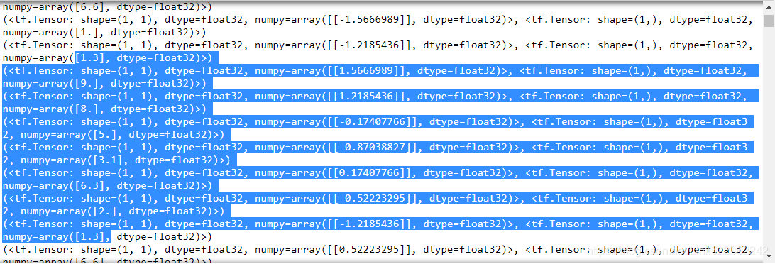
####################################
Let's look at the trained model and plot it. For test data, we will create a NumPy array of values evenly spaced均匀分布 between 0 to 9. Since we trained our model with standardized features, we will also apply the same standardization to the test data:
print( 'Final Parameters:', model.w.numpy(), model.b.numpy() )

X_test = np.linspace( 0,9, num=100).reshape(-1,1)
X_test_norm = ( X_test -np.mean(X_train) )/np.std(X_train)

y_pred = model( tf.cast(X_test_norm, dtype=tf.float32) )

fig = plt.figure( figsize=(13,5) )

ax = fig.add_subplot(1,2,1)
plt.plot(X_train_norm, y_train, 'o', markersize=10)
plt.plot(X_test_norm, y_pred, '--', lw=3)
plt.legend( ['Training examples', 'Linear Reg.'],
            fontsize=15 )
ax.set_xlabel('x', size=15)
ax.set_ylabel('y', size=15)
ax.tick_params( axis='both', which='major', labelsize=15 )

ax = fig.add_subplot(1,2,2)
plt.plot(Ws, lw=3)
plt.plot(bs, lw=3)
plt.legend(['Weight w', 'Bias unit b'], fontsize=15)
ax.set_xlabel('Iteration', size=15)
ax.set_ylabel('Value', size=15)
ax.tick_params(axis='both', which='major', labelsize=15)

plt.show()
The following figure shows the scatterplot of the training examples and the trained linear regression model, as well as the convergence history of the weight, w, and the
bias unit, b: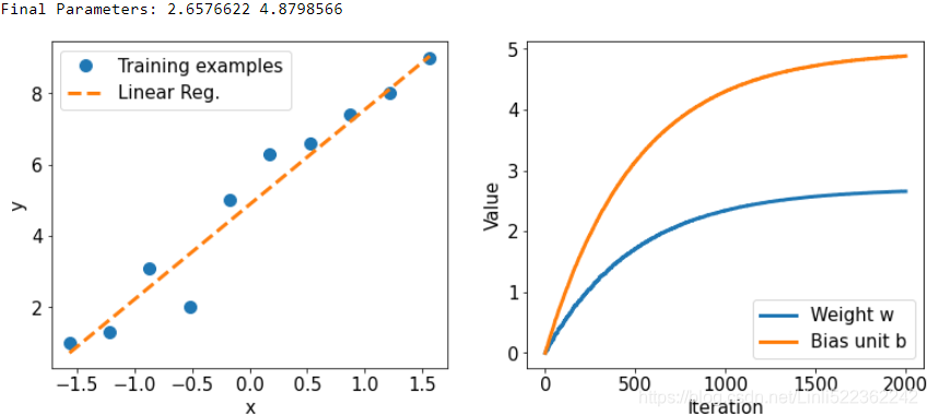
Model training via the .compile() and .fit() methods
In the previous example, we saw how to train a model by writing a custom function, train(), and applied stochastic gradient descent optimization. However, writing the train() function can be a repeatable task across different projects. The TensorFlow Keras API provides a convenient .fit() method that can be called on an instantiated model. To show how this works, let's create a new model and compile it by selecting the optimizer, loss function, and evaluation metrics:
tf.random.set_seed(1)
model = MyModel()

model.compile( optimizer='sgd', loss=loss_fn, metrics=['mae', 'mse'])
Now, we can simply call the fit() method to train the model. We can pass a batched dataset (like ds_train, which was created in the previous example). However, this
time you will see that we can pass the NumPy arrays for x and y directly, without needing to create a dataset:
# batch_size = 1
# num_epochs = 200
model.fit(X_train_norm, y_train, epochs=num_epochs, batch_size=batch_size, verbose=1)
# verbose=1 : Output 1 line of log information for each epoch in the standard output stream
# 10/10 use whole dataset( len(dataset)==10 ) # 12 _Custom Models and Training with TensorFlow_2_progress_status_bar_Training Loops_concrete https://blog.csdn.net/Linli522362242/article/details/107459161
total number of '=' : p=size-1 and size=30 https://blog.csdn.net/Linli522362242/article/details/107459161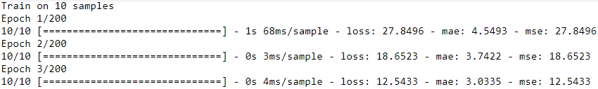
......
After the model is trained, visualize the results and make sure that they are similar to the results of the previous method.
Building a multilayer perceptron for classifying flowers in the Iris dataset
In the previous example, you saw how to build a model from scratch. We trained this model using stochastic gradient descent optimization. While we started our journey based on the simplest possible example, you can see that defining the model from scratch, even for such a simple case, is neither appealing nor a good practice. TensorFlow instead provides already defined layers through tf.keras.layers that can be readily used as the building blocks of an NN model. In this section, you will learn how to use these layers to solve a classification task using the Iris flower dataset and build a two-layer perceptron using the Keras API. First, let's get the data from tensorflow_datasets:
################################
C:\Anaconda3\envs\tensorflow\Lib\site-packages\tensorflow_datasets\image_classification
class Iris(tfds.core.GeneratorBasedBuilder):
  """Iris flower dataset."""
  NUM_CLASSES = 3
#  VERSION = tfds.core.Version(
#      "2.0.0", "New split API (https://tensorflow.org/datasets/splits)")
  VERSION = tfds.core.Version("1.0.0")
  SUPPORTED_VERSIONS = [
      tfds.core.Version("2.0.0", "EXP1: Opt-in for experiment 1",
                        experiments={tfds.core.Experiment.EXP1: True}),
  ]
...
import tensorflow_datasets as tfds
iris, iris_info = tfds.load('iris:1.0.0')
print(iris_info)
C:\Anaconda3\envs\tensorflow\Lib\site-packages\tensorflow_datasets\image_classification
change back
class Iris(tfds.core.GeneratorBasedBuilder):
  """Iris flower dataset."""
  NUM_CLASSES = 3
  VERSION = tfds.core.Version(
      "2.0.0", "New split API (https://tensorflow.org/datasets/splits)")
...
import tensorflow_datasets as tfds
iris, iris_info = tfds.load('iris:2.0.0', with_info=True)
print(iris_info)
################################
Is the version of mnist 2.0.0?
import tensorflow_datasets as tfds

iris, iris_info = tfds.load('iris', with_info=True)
# iris, iris_info = tfds.load('iris:2.0.0', with_info=True)
print(iris_info)
Yes:

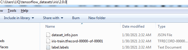
This prints some information about this dataset. However, you will notice in the shown information that this dataset comes with only one partition(  VS
VS  ), so we have to split the dataset into training and testing partitions (and validation for proper machine learning practice) on our own. Let's assume that we want to use two-thirds of the dataset for training and keep the remaining examples for testing. The tensorflow_datasets library provides a convenient tool that allows us to determine slices and splits via the DatasetBuilder object prior to loading a dataset. You can find out more about splits at https://www.tensorflow.org/datasets/splits.
iris['train']![]()
An alternative approach is to load the entire dataset first and then use .take() and .skip() to split the dataset to two partitions. If the dataset is not shuffled at first, we can also shuffle the dataset. However, we need to be very careful with this because it can lead to mixing the train/test examples, which is not acceptable in machine learning. To avoid this, we have to set an argument, reshuffle_each_iteration=False, in the .shuffle() method. The code for splitting the dataset into train/test is as follows:
import tensorflow as tf

tf.random.set_seed(1)

ds_orig = iris['train']
ds_orig = ds_orig.shuffle(150, reshuffle_each_iteration=False)############

print( next(iter(ds_orig)) )

ds_train_orig = ds_orig.take(100) # size=100
ds_test = ds_orig.skip(100) # size=50![]()
Next, as you have already seen in the previous sections, we need to apply a transformation via the .map() method to convert the dictionary to a tuple:
ds_train_orig = ds_train_orig.map( lambda x: (x['features'], x['label']) )
ds_test = ds_test.map( lambda x: (x['features'], x['label']) )

ds_train_orig![]()
next( iter(ds_train_orig) )![]()
Now, we are ready to use the Keras API to build a model efficiently. In particular, using the tf.keras.Sequential class, we can stack a few Keras layers and build an
NN. You can see the list of all the Keras layers that are already available at https://www.tensorflow.org/versions/r2.0/api_docs/python/tf/keras/layers. For this problem, we are going to use the Dense layer (tf.keras.layers.Dense), which is also known as a fully connected (FC) layer or linear layer, and can be best represented by 𝑓(𝑤 × 𝑥 + 𝑏) , where x is the input features, w and b are the weight matrix and the bias vector, and f is the activation function.
# checking the number of examples:
n=0
for example in ds_train_orig:
    n += 1
print(n)

n=0
for example in ds_test:
    n += 1
print(n)![]()
If you think of the layers in an NN, each layer receives its inputs from the preceding layer; therefore, its dimensionality (rank and shape) is fixed. Typically, we need to concern ourselves with the dimensionality of output only when we design an NN architecture. (Note: the first layer is the exception, but TensorFlow/Keras allows us to decide the input dimensionality of the first layer after defining the model through late variable creation.) Here, we want to define a model with two hidden layers. The first one receives an input of four features and projects them to 16 neurons. The second layer receives the output of the previous layer (which has size 16) and projects them to three output neurons, since we have three class labels. This can be done using the Sequential class and the Dense layer in Keras as follows:
##############################################
why we use sigmoid?
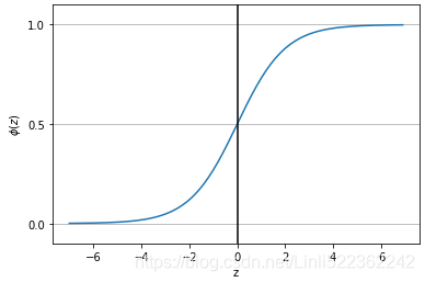
Advantages: non-linear; limited output range, suitable for output layer.
Disadvantages: too smooth on both sides, and the learning rate is too low; the value is always positive; the output is not centered at 0.
Applicable to: When we try to classify values into specific classes, using the Sigmoid function is ideal.
why we use exponential
an exponential function:
 Note a=e,
For each class (either e^x<0, or e^x>0; that is to say, the activation function is classified according to (current network layer output>0 or output<0), we only consider the output when it is greater than 0 value
iris_model = tf.keras.Sequential([
    tf.keras.layers.Dense( 16, activation='sigmoid', name='fc1', input_shape=(4,) ),
    tf.keras.layers.Dense( 3, name = 'fc2', activation='softmax')
])
iris_model.summary()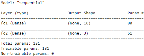
Notice that we determined the input shape for the first layer via input_shape=(4,), and therefore, we did not have to call .build() anymore in order to use iris_model.summary().
The printed model summary indicates that the first layer (fc1) has 80 parameters(=(4+1)x16=80), and the second layer has 51 parameters(=(16+1)x3=51). You can verify that by ![]() , where
, where ![]() is the number of input units, and
is the number of input units, and ![]() is the number of output units. Recall that for a fully (densely) connected layer, the learnable parameters are the weight matrix of size
is the number of output units. Recall that for a fully (densely) connected layer, the learnable parameters are the weight matrix of size ![]() and the bias vector of size
and the bias vector of size ![]() . Furthermore, notice that we used the sigmoid activation function for the first layer and softmax activation###################################
. Furthermore, notice that we used the sigmoid activation function for the first layer and softmax activation###################################
(Equation 4-19. Softmax score for class k ![]()
Note that each class has its own dedicated parameter vector ![]() . All these vectors are typically stored as rows in a parameter matrix
. All these vectors are typically stored as rows in a parameter matrix ![]() . Note
. Note ![]() ==b
==b
[ #class0, class1, ...., classN
[b0==1, b0==1, ... repeat...],
[b1, b1, ..., repeat...],
... ...
[bk, bk, ... repeat...]
]
Theta: (number_of_theta=features plus the bias term , number of label names/class )![]() : (number of label names/class , number_of_theta
: (number of label names/class , number_of_theta![]() =features plus the bias term )
=features plus the bias term )
X_train( number of features plus the bias term, number of instances): one column is a instance,
[ [x_b0==1, x_b0==1, ... repeat...], [x_b1, x_b1, ... repeat...], ..., [x_bk, x_bk, ... repeat...]]
logits = ![]() :
: ![]() ; p is corresponding to features including bias/intercept
; p is corresponding to features including bias/intercept
Once you have computed the score of every class for the instance x, you can estimate the probability ![]() that the instance belongs to class k by running the scores through the softmax function (Equation 4-20): it computes the exponential of every score(), then normalizes them (dividing by the sum of all the exponentials).
that the instance belongs to class k by running the scores through the softmax function (Equation 4-20): it computes the exponential of every score(), then normalizes them (dividing by the sum of all the exponentials).
==> Equation 4-20. Softmax function 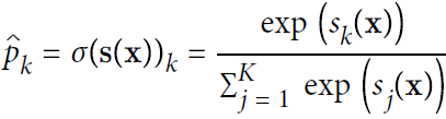
• K is the number of classes.
• s(x) is a vector containing the scores of each class for the instance x.
•![]() is the estimated probability that the instance x belongs to class k given the scores of each class for that instance.
is the estimated probability that the instance x belongs to class k given the scores of each class for that instance.
Just like the Logistic Regression classifier, the Softmax Regression classifier predicts the class with the highest estimated probability (which is simply the class with the highest score), as shown in Equation 4-21.
Equation 4-21. Softmax Regression classifier prediction ![]()
The argmax operator returns the value of a variable that maximizes a function. In this equation, it returns the value of k that maximizes the estimated probability ![]() .
.
return index/k max of ==> return index/k max of ![]()
![]() is a weight vector: Theta = Theta - eta*gradients
is a weight vector: Theta = Theta - eta*gradients
###04_TrainingModels_04_gradient decent with early stopping for softmax regression_ entropy_Gini : https://blog.csdn.net/Linli522362242/article/details/104124771
###################################) for the last (output) layer. Softmax activation in the last layer is used to support multi-class classification, since here we have three class labels (which is why we have three neurons at the output layer). We will discuss the different activation functions and their applications later in this chapter.
Next, we will compile this model to specify the loss function, the optimizer, and the metrics for evaluation:
######################
adam? https://blog.csdn.net/Linli522362242/article/details/106982127 ~~~https://blog.csdn.net/Linli522362242/article/details/107086444
To reduce the loss function, the error between the true value and the predicted value is reduced (or the predicted value is close to the true value)

Recall that Gradient Descent updates the weights θ by directly subtracting the gradient of the cost function J(θ) with regard to the weights (![]() ) multiplied by the learning rate η. The equation is: θ ← θ –
) multiplied by the learning rate η. The equation is: θ ← θ – ![]() OR
OR 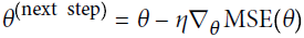 https://blog.csdn.net/Linli522362242/article/details/104005906. It does not care about what the earlier gradients were. If the local gradient is tiny, it goes very slowly.
http://www.cs.toronto.edu/~hinton/absps/momentum.pdf
Equation 11-4. Momentum algorithm : 11_Training Deep NN_2_transfer learning_split_datase_RBMs_Momentum_Nesterov AccelerG_AdaGrad_RMSProphttps://blog.csdn.net/Linli522362242/article/details/106982127
 # it subtracts the local gradient * η from the momentum vector m, m is negative
 # it updates the weights by adding this momentum vector m, note m is negative
Momentum optimization cares a great deal about what previous gradients were: at each iteration, it subtracts the local gradient from the momentum vector m (multiplied by the learning rate η), and it updates the weights by adding this momentum vector (see Equation 11-4). In other words, the gradient is used for acceleration, not for speed. To simulate some sort of friction摩擦 mechanism and prevent the momentum m from growing too large, the algorithm introduces a new hyperparameter β, called the momentum, which must be set between 0 (high friction) and 1 (no friction). A typical momentum value is 0.9.
You can easily verify that if the gradient remains constant, the terminal velocity (i.e., the maximum size of the weight updates) is equal to that gradient multiplied by the learning rate η multiplied by 1/(1–β) (ignoring the sign).### ![]() VS
VS ![]() and 0<= β <1
and 0<= β <1 
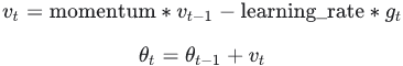
In keras:
The update rule for θ with gradient g when momentum(β) is 0.0:![]()
The update rule when momentum is larger than 0.0(β>0): ![]() is negative since
is negative since ![]() ,有方向的gradent是向下(negative),但是在计算机计算过程为了好处理使用了正值, 因此
,有方向的gradent是向下(negative),但是在计算机计算过程为了好处理使用了正值, 因此![]()
if nesterov is False, gradient is evaluated at ![]() .
.
if nesterov is True, gradient is evaluated at ![]() , and the variables always store θ+mv instead of theta
, and the variables always store θ+mv instead of theta
Nesterov Accelerated Gradient : https://blog.csdn.net/Linli522362242/article/details/106982127
One small variant to momentum optimization, proposed by Yurii Nesterov in 1983,14 is almost always faster than vanilla momentum optimization. The Nesterov Accelerated Gradient (NAG) method, also known as Nesterov momentum optimization, measures the gradient of the cost function not at the local position θ but slightly ahead in the direction of the momentum, at θ + βm (see Equation 11-5) OR ![]() .
.
Equation 11-5. Nesterov Accelerated Gradient algorithm
This small tweak works because in general the momentum vector m will be pointing in the right direction (i.e., toward the optimum), so it will be slightly more accurate to use the gradient measured a bit farther in that direction rather than using the gradient at the original position, as you can see in Figure 11-6 (where ![]() represents the gradient of the cost function measured at the starting point θ, and
represents the gradient of the cost function measured at the starting point θ, and ![]() represents the gradient at the point located at θ + βm, Note: θ*βm<0).
represents the gradient at the point located at θ + βm, Note: θ*βm<0). 

Figure 11-6. Regular versus Nesterov Momentum optimization(![]() ==β); the former applies the gradients
==β); the former applies the gradients ![]() computed before the momentum step(βm), while the latter applies the gradients
computed before the momentum step(βm), while the latter applies the gradients![]() ###
###![]() ### computed after.
### computed after.
As you can see, the Nesterov update ends up slightly closer to the optimum. After a while, these small improvements add up and NAG ends up being significantly faster than regular Momentum optimization. Moreover, note that when the momentum pushes the weights across a valley, ![]() continues to push further across the valley, while
continues to push further across the valley, while ![]() pushes back toward the bottom of the valley(更正方向). This helps reduce oscillations and thus converges faster(Nesterov Accelerated Gradient).
pushes back toward the bottom of the valley(更正方向). This helps reduce oscillations and thus converges faster(Nesterov Accelerated Gradient).
AdaGrad (is well-suited for dealing with sparse data)
Figure 11-7. AdaGrad versus Gradient Descent: the former can correct its direction earlier to point to the optimum

Consider the elongated bowl problem again: Gradient Descent starts by quickly going down the steepest slope, which does not point straight toward the global optimum, then it very slowly goes down to the bottom of the valley. It would be nice if the algorithm could correct its direction earlier to point a bit more toward the global optimum. The AdaGrad algorithm achieves this correction by scaling down the gradient vector along the steepest dimensions (see Equation 11-6).
https://ruder.io/optimizing-gradient-descent/index.html#fn12 Adagradis an algorithm for gradient-based optimization that does just this: It adapts the learning rate to the parameters, performing smaller updates
(i.e. low learning rates) for parameters associated with frequently occurring features, and larger updates (i.e. high learning rates) for parameters associated with infrequent features. For this reason, it is well-suited for dealing with sparse data. Dean et al. [10] have found that Adagrad greatly improved the robustness of SGD and used it for training large-scale neural nets at Google, which -- among other things -- learned to recognize cats in Youtube videos. Moreover, Pennington et al. [11] used Adagrad to train GloVe word embeddings, as infrequent words require much larger updates than frequent ones.
Previously, we performed an update for all parameters θ at once as every parameter ![]() used the same learning rate η. As Adagrad uses a different learning rate for every parameter
used the same learning rate η. As Adagrad uses a different learning rate for every parameter ![]() at every time step t (consider steps_per_epoch*num_epochs OR How many steps are used to train whole training datasets in each epoch), we first show Adagrad's per-parameter update, which we then vectorize. For brevity, we use
at every time step t (consider steps_per_epoch*num_epochs OR How many steps are used to train whole training datasets in each epoch), we first show Adagrad's per-parameter update, which we then vectorize. For brevity, we use ![]() to denote the gradient at time step t.
to denote the gradient at time step t. ![]() is then the partial derivative of the objective function w.r.t.(with regard to) to the parameter
is then the partial derivative of the objective function w.r.t.(with regard to) to the parameter ![]() at time step t:
at time step t:![]()
The SGD update for every parameter ![]() at each time step t then becomes:
at each time step t then becomes: ![]()
In its update rule, Adagrad modifies the general learning rate η at each time step t for every parameter ![]() based on the past gradients that have been computed for
based on the past gradients that have been computed for ![]() :
:
![]() here is a diagonal matrix where each diagonal element i,i is the sum of the squares of the gradients w.r.t.
here is a diagonal matrix where each diagonal element i,i is the sum of the squares of the gradients w.r.t. ![]() up to time step t (每个对角线位置i,i为对应参数
up to time step t (每个对角线位置i,i为对应参数![]() 从第1_step到第t_step梯度的平方和
从第1_step到第t_step梯度的平方和 OR
OR ![]() ), while ϵ is a smoothing term that avoids division by zero (usually on the order of 1e−8). Interestingly, without the square root operation, the algorithm performs much worse. Adagrad的缺点是在训练的中后期,分母上梯度平方的累加将会越来越大,从而梯度
), while ϵ is a smoothing term that avoids division by zero (usually on the order of 1e−8). Interestingly, without the square root operation, the algorithm performs much worse. Adagrad的缺点是在训练的中后期,分母上梯度平方的累加将会越来越大,从而梯度 趋近于0,使得训练提前结束。.
As ![]() contains the sum of the squares of the past gradients w.r.t. to all parameters θ along its diagonal, we can now vectorize our implementation by performing a matrix-vector product ⊙ between
contains the sum of the squares of the past gradients w.r.t. to all parameters θ along its diagonal, we can now vectorize our implementation by performing a matrix-vector product ⊙ between ![]() and
and ![]() :
:
One of Adagrad's main benefits is that it eliminates the need to manually tune the learning rate. Most implementations use a default value of 0.01 and leave it at that.
Adagrad's main weakness is its accumulation of the squared gradients in the denominator: Since every added term is positive, the accumulated sum keeps growing![]() OR during training. This in turn causes the learning rate to shrink and eventually become infinitesimally smallAdaGrad runs the risk of slowing down a bit too fast and never converging to the global optimum, at which point the algorithm is no longer able to acquire additional knowledge. The following algorithms aim to resolve this flaw.
OR during training. This in turn causes the learning rate to shrink and eventually become infinitesimally smallAdaGrad runs the risk of slowing down a bit too fast and never converging to the global optimum, at which point the algorithm is no longer able to acquire additional knowledge. The following algorithms aim to resolve this flaw.
Equation 11-6. AdaGrad algorithm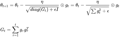
 # accumulates s 约束项regularizer: 1/

特点:
- 前期accumulates较小的时候, regularizer较大,能够放大梯度
- 后期accumulates较大的时候,regularizer较小,能够约束梯度
- 适合处理稀疏梯度
缺点:
- 由公式可以看出,仍依赖于人工设置一个全局学习率
- learning rate设置过大的话,会使regularizer过于敏感,对梯度的调节太大
- 中后期,分母上梯度平方的累加将会越来越大,使
 -->0,使gradent-->0,使得训练提前结束
The first step accumulates the square of the gradients into the vector s (recall that the ⊗ symbol represents the element-wise multiplication![]() ). This vectorized form is equivalent to computing
). This vectorized form is equivalent to computing ![]() for each element
for each element ![]() of the vector s; in other words, each
of the vector s; in other words, each ![]() accumulates the squares of the partial derivative of the cost function with regard to parameter
accumulates the squares of the partial derivative of the cost function with regard to parameter ![]() . If the cost function is steep along the
. If the cost function is steep along the ![]() dimension, then
dimension, then![]() will get larger and larger at each iteration.
will get larger and larger at each iteration.
The second step is almost identical to Gradient Descent, but with one big difference: the gradient vector is scaled down by a factor of s + ε (the ⊘ symbol represents the element-wise division, and ε is a smoothing term to avoid division by zero, typically set to ![]() ). This vectorized form is equivalent to simultaneously computing
). This vectorized form is equivalent to simultaneously computing ![]() for all parameters
for all parameters ![]() .
.
In short, this algorithm decays the learning rate, but it does so faster for steep dimensions than for dimensions with gentler slopes. This is called an adaptive learning rate. It helps point the resulting updates more directly toward the global optimum (see Figure 11-7). One additional benefit is that it requires much less tuning of the learning rate hyperparameter η.
RMSProp (RootMeanSquareProp) https://ruder.io/optimizing-gradient-descent/index.html#fn12
As we’ve seen, AdaGrad runs the risk of slowing down a bit too fast and never converging to the global optimum. The RMSProp algorithm fixes this by accumulating only the gradients from the most recent iterations (as opposed to all the gradients since the beginning of training). It does so by using exponential decay in the first step (see Equation 11-7).
Equation 11-7. RMSProp algorithm vs AdaGrad
The decay rate β is typically set to 0.9. Yes, it is once again a new hyperparameter, but this default value often works well, so you may not need to tune it at all.

RMSprop as well divides the learning rate by an exponentially decaying average of squared gradients. Hinton suggests γ to be set to 0.9, while a good default value for the learning rate η is 0.001.
Adam > RMSprop > Adagrad
https://ruder.io/optimizing-gradient-descent/index.html#fn12 and https://blog.csdn.net/u010089444/article/details/76725843
Adaptive Moment Estimation (Adam) is another method that computes adaptive learning rates for each parameter. In addition to storing an exponentially decaying average of past squared gradients ![]() like Adadelta and RMSprop, Adam also keeps an exponentially decaying average of past gradients
like Adadelta and RMSprop, Adam also keeps an exponentially decaying average of past gradients ![]() , similar to momentum. Whereas momentum can be seen as a ball running down a slope, Adam behaves like a heavy ball with friction, which thus prefers flat minima in the error surface. We compute the decaying averages of past
, similar to momentum. Whereas momentum can be seen as a ball running down a slope, Adam behaves like a heavy ball with friction, which thus prefers flat minima in the error surface. We compute the decaying averages of past![]() and past squared gradients
and past squared gradients![]() respectively as follows:
respectively as follows: <==
<== ![]() and
and ![]()
![]() and v_t are estimates of the first moment (the mean) and the second moment (the uncentered variance) of the gradients respectively,
and v_t are estimates of the first moment (the mean) and the second moment (the uncentered variance) of the gradients respectively, ![]() ,
,![]() 分别是对梯度的一阶矩估计和二阶矩估计,可以看作对
分别是对梯度的一阶矩估计和二阶矩估计,可以看作对![]() 的近似, hence the name of the method. As
的近似, hence the name of the method. As ![]() and
and ![]() are initialized as vectors of 0's, the authors of Adam observe that they are biased towards zero, especially during the initial time steps, and especially when the decay rates are small (i.e. β1 and β2 are close to 1).
are initialized as vectors of 0's, the authors of Adam observe that they are biased towards zero, especially during the initial time steps, and especially when the decay rates are small (i.e. β1 and β2 are close to 1).
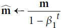
They counteract抵消 these biases by computing bias-corrected first and second moment estimates: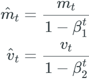
They then use these to update the parameters just as we have seen in Adadelta and RMSprop, which yields the Adam update rule: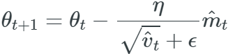
The authors propose default values of 0.9 for β1, 0.999 for β2, and ![]() for ϵ. They show empirically that Adam works well in practice and compares favorably to other adaptive learning-method algorithms.
for ϵ. They show empirically that Adam works well in practice and compares favorably to other adaptive learning-method algorithms.
Adam, which stands for adaptive moment estimation自适应矩估计, combines the ideas of momentum optimization and RMSProp: just like momentum optimization, it keeps track of an exponentially decaying average of past gradients; and just like RMSProp, it keeps track of an exponentially decaying average of past squared gradients (see Equation 11-8).
Equation 11-8. Adam algorithm
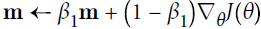 # Momentum algorithm #1
 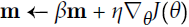 β, called the momentum prevent the momentum m from growing too large(A typical momentum value is 0.9)
 # RMSProp algorithm #1

 # RMSProp algorithm 2#2
- In this equation, t represents the iteration number (starting at 1).
- 在数据比较稀疏的时候,adaptive的方法能得到更好的效果,例如Adagrad,RMSprop, Adam 等。Adam 方法也会比 RMSprop方法收敛的结果要好一些, 所以在实际应用中 ,Adam为最常用的方法,可以比较快地得到一个预估结果。
############
Losses and metrics are conceptually not the same thing: losses (e.g., cross entropy) are used by Gradient Descent to train a model, so they must be differentiable (at least where they are evaluated), and their gradients should not be 0 everywhere. Plus, it’s OK if they are not easily interpretable by humans. In contrast, metrics (e.g., accuracy) are used to evaluate a model: they must be more easily interpretable, and they can be non-differentiable or have 0 gradients everywhere.https://blog.csdn.net/Linli522362242/article/details/107294292 https://blog.csdn.net/Linli522362242/article/details/108414534
loss = 'sparse_categorical_crossentropy' ==> optimizer='adam',
iris_model.compile( optimizer='adam',
                    loss = 'sparse_categorical_crossentropy',
                    metrics=['accuracy'] ) #<== classification
Now, we can train the model. We will specify the number of epochs to be 100 and the batch size to be 2. In the following code, we will build an infinitely repeating dataset, which will be passed to the fit() method for training the model. In this case, in order for the fit() method to be able to keep track of the epochs, it needs to know the number of steps for each epoch.
Given the size of our training data (here, 100) and the batch size (batch_size), we can determine the number of steps in each epoch, steps_per_epoch:
num_epochs = 100
training_size = 100
batch_size = 2
steps_per_epoch = np.ceil( training_size/batch_size )

ds_train = ds_train_orig.shuffle( buffer_size=training_size )
ds_train = ds_train.repeat() #infinitely repeating dataset
ds_train = ds_train.batch( batch_size=batch_size )
ds_train = ds_train.prefetch( buffer_size=1000 )

history = iris_model.fit( ds_train, epochs=num_epochs,
                          steps_per_epoch = steps_per_epoch,
                          verbose=0 )
hist = history.history
import matplotlib.pyplot as plt
%matplotlib inline
fig = plt.figure( figsize=(12,5) )
ax = fig.add_subplot(1,2,1)
ax.plot( hist['loss'], lw=3 ) # len( hist['loss'] )==100
ax.set_title('Training loss', size=15)
ax.set_xlabel('Epoch', size=15)
# axis{'x', 'y', 'both'}, default: 'both' : The axis to which the parameters are applied.
# which{'major', 'minor', 'both'}, default: 'major' The group of ticks to which the parameters are applied.
ax.tick_params( axis='both', which='major', labelsize=15)
ax = fig.add_subplot(1,2,2)
ax.plot( hist['accuracy'], lw=3)
ax.set_title('Train accuracy', size=15)
ax.set_xlabel('Epoch', size=15)
ax.tick_params( axis='both', which='minor', labelsize=15)The learning curves (training loss and training accuracy) are as follows:

Evaluating the trained model on the test dataset
Since we specified 'accuracy' as our evaluation metric in iris_model.compile(), we can now directly evaluate the model on the test dataset:
# ds_test.batch(50) ==> <BatchDataset shapes: ((None, 4), (None,)), types: (tf.float32, tf.int64)>
# ds_test = ds_orig.skip(100)
# ds_test.batch(50) ==> <BatchDataset shapes: ((None, 4), (None,)), types: (tf.float32, tf.int64)>
results = iris_model.evaluate( ds_test.batch(50), verbose=0)
print('Test loss: {:.4f} Test Acc.: {:.4f}'.format(*results))![]()
Notice that we have to batch the test dataset as well, to ensure that the input to the model has the correct dimension (rank). As we discussed earlier, calling .batch()
will increase the rank of the retrieved tensors by 1. The input data for .evaluate() must have one designated dimension for the batch(num_of_samples), although here (for evaluation), the size of the batch does not matter. Therefore, if we pass ds_batch.batch(50) to the .evaluate() method, the entire test dataset will be processed in one batch of size 50, but if we pass ds_batch.batch(1), 50 batches of size 1 will be processed.
# ds_test = ds_orig.skip(100)
# ds_test.batch(50) ==> <BatchDataset shapes: ((None, 4), (None,)), types: (tf.float32, tf.int64)>
results = iris_model.evaluate( ds_test.batch(1), verbose=0)
# results ==> [0.1483253389596939, 0.98]
print('Test loss: {:.4f} Test Acc.: {:.4f}'.format(*results))![]()
Saving and reloading the trained model
Trained models can be saved on disk for future use. This can be done as follows:
iris_model.save( 'iris-classifier.h5',
                 overwrite=True,
                 include_optimizer=True,
save_format='h5')![]()
The first option is the filename. Calling iris_model.save() will save both the model architecture and all the learned parameters(Weights). However, if you want to save only the architecture, you can use the iris_model.to_json() method, which saves the model configuration in JSON format. Or if you want to save only the model weights, you can do that by calling iris_model.save_weights(). The save_format can be specified to be either 'h5' for the HDF5 format or 'tf' for TensorFlow format.
iris_model.to_json() 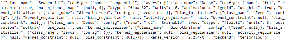
Now, let's reload the saved model. Since we have saved both the model architecture and the weights, we can easily rebuild and reload the parameters in just one line; Try to verify the model architecture by calling iris_model_new.summary().
iris_model_new = tf.keras.models.load_model('iris-classifier.h5')

iris_model_new.summary()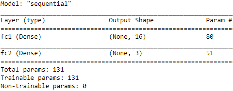
Finally, let's evaluate this new model that is reloaded on the test dataset to verify that the results are the same as before:
results = iris_model_new.evaluate( ds_test.batch(50), verbose=0 )
# results ==> [0.1483253389596939, 0.98]
print( 'Test loss: {:.4f} Test Acc.: {:.4f}'.format(*results) )![]()
labels_train = []
# ds_train_orig : <MapDataset shapes: ((4,), ()), types: (tf.float32, tf.int64)>
for i, item in enumerate( ds_train_orig ):
    labels_train.append( item[1].numpy() )

labels_test = []
for i, item in enumerate( ds_test ):
    labels_test.append( item[1].numpy() )

print('Training Set: ', len(labels_train), \
'Test Set: ', len(labels_test) )![]()
Choosing activation functions for multilayer neural networks
For simplicity, we have only discussed the sigmoid activation function in the context of multilayer feedforward NNs so far; we used it in the hidden layer as well as the
output layer in the MLP implementation in cp12, Implementing a Multilayer Artificial Neural_gzip_mnist_struct_savez_compressed_fetch_openml_back propagation_weight update_L2 https://blog.csdn.net/Linli522362242/article/details/111940633.
Note that in this book, the sigmoidal logistic function, ![]() , is referred to as the sigmoid function for brevity, which is common in machine learning literature. In the following subsections, you will learn more about alternative nonlinear functions that are useful for implementing multilayer NNs.
, is referred to as the sigmoid function for brevity, which is common in machine learning literature. In the following subsections, you will learn more about alternative nonlinear functions that are useful for implementing multilayer NNs.
Technically, we can use any function as an activation function in multilayer NNs as long as it is differentiable. We can even use linear activation functions, such as in Adaline (Chapter 2, Training Simple Machine Learning Algorithms for Classification https://blog.csdn.net/Linli522362242/article/details/96429442). However, in practice, it would not be very useful to use linear activation functions for both hidden and output layers, since we want to introduce nonlinearity in a typical artificial NN to be able to tackle complex problems. The sum of linear functions yields a linear function after all.
The logistic (sigmoid) activation function that we used in cp12 probably mimics the concept of a neuron in a brain most closely—we can think of it as the probability of whether a neuron fires. However, the logistic (sigmoid) activation function can be problematic if we have highly negative input, since the output of the sigmoid function will be close to zero in this case. If the sigmoid function returns output that is close to zero, the NN will learn very slowly, and it will be more likely to get trapped in the local minima during training. This is why people often prefer a hyperbolic tangent as an activation function in hidden layers.
Before we discuss what a hyperbolic tangent looks like, let's briefly recapitulate [ˌri:kəˈpɪtʃuleɪt]重述 some of the basics of the logistic function and look at a generalization that makes it more useful for multilabel classification problems.
Logistic function recap
As was mentioned in the introduction to this section, the logistic function is, in fact, a special case of a sigmoid function. You will recall from the section on logistic regression in Chapter 3, A Tour of Machine Learning Classifiers Using scikit-learn https://blog.csdn.net/Linli522362242/article/details/96480059, that we can use a logistic function to model the probability that sample x belongs to the positive class (class 1) in a binary classification task.
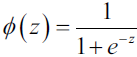
The given net input, z, is shown in the following equation: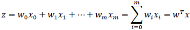
The logistic (sigmoid) function will compute the following: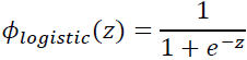
Note that ![]() is the bias unit (y-axis intercept, which means
is the bias unit (y-axis intercept, which means ![]() ). To provide a more concrete example, let's take a model for a two-dimensional data point, x, and a model with the following weight coefficients assigned to the w vector:
). To provide a more concrete example, let's take a model for a two-dimensional data point, x, and a model with the following weight coefficients assigned to the w vector:
import numpy as np

X = np.array([1, 1.4, 2.5]) # first value must be 1
w = np.array([0.4, 0.3, 0.5])

def net_input(X, w):
    return np.dot(X,w)

def logistic(z):
    return 1.0 / (1.0+np.exp(-z))

def logistic_activation(X, w):
    z = net_input(X,w)
    return logistic(z)

print('P(y=1|x) = %.3f' % logistic_activation(X,w))![]()
If we calculate the net input (z) and use it to activate a logistic neuron with those particular feature values and weight coefficients, we get a value of 0.888, which we can interpret as an 88.8 percent probability that this particular sample, x, belongs to the positive class.
In Chapter 12, we used the one-hot encoding technique to represent multiclass ground truth labels and designed the output layer consisting of multiple logistic activation units. However, as will be demonstrated by the following code example, an output layer consisting of multiple logistic activation units does not produce meaningful, interpretable probability values:
# W: array with shape = (n_output_units, n_hidden_units+1)
# note that the first column are the bias units
              #w_0, w_1, w_2, w_3
W = np.array([[1.1, 1.2, 0.8, 0.4],
              [0.2, 0.4, 1.0, 0.2],
              [0.6, 1.5, 1.2, 0.7]])

# A: data array with shape = (n_hidden_units+1, n_samples)
# note that the first column of this array must be 1
A = np.array([[1, 0.1, 0.4, 0.6]])
Z = np.dot(W, A[0])
y_probas = logistic(Z)

print('Net Input: \n', Z)
print('Output Units:\n', y_probas)
As you can see in the output, the resulting values cannot be interpreted as probabilities for a three-class problem. The reason for this is that they do not sum up to 1. However, this is, in fact, not a big concern if we use our model to predict only the class labels and not the class membership probabilities. One way to predict the class label from the output units obtained earlier is to use the maximum value:
# W: array with shape = (n_output_units, n_hidden_units+1)
# W: array with shape = (n_output_units, n_hidden_units+1)
# note that the first column are the bias units
              #w_0, w_1, w_2, w_3
W = np.array([[1.1, 1.2, 0.8, 0.4],
              [0.2, 0.4, 1.0, 0.2],
              [0.6, 1.5, 1.2, 0.7]])

# A: data array with shape = (n_hidden_units+1, n_samples)
# note that the first column of this array must be 1
A = np.array([[1, 0.1, 0.4, 0.6]])
Z = np.dot(W, A[0])
y_probas = logistic(Z)

print('Net Input: \n', Z)
print('Output Units:\n', y_probas)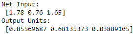
y_class = np.argmax(Z, axis=0)
print('Predicted class label: %d' % y_class)![]()
In certain contexts, it can be useful to compute meaningful class probabilities for multiclass predictions. In the next section, we will take a look at a generalization of the logistic function, the softmax function, which can help us with this task.
Estimating class probabilities in multiclass classification via the softmax function
In the previous section, you saw how we can obtain a class label using the argmax function. Previously, in the section Building a multilayer perceptron for classifying flowers in the Iris dataset, we determined activation='softmax' in the last layer of the MLP model. The softmax function is a soft form of the argmax function; instead of giving a single class index, it provides the probability of each class. Therefore, it allows us to compute meaningful class probabilities in multiclass settings (multinomial logistic regression).
In softmax, the probability of a particular sample with net input z belonging to the ith class can be computed with a normalization term in the denominator, that is, the sum of the exponentially weighted linear functions:
To see softmax in action, let's code it up in Python:
def softmax(z):
    return np.exp(z) / np.sum( np.exp(z) )

y_probas = softmax(Z)
print( 'Probabilities:\n', y_probas )

np.sum(y_probas)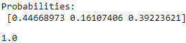
As you can see, the predicted class probabilities now sum up to 1, as we would expect. It is also notable that the predicted class label is the same as when we applied the argmax function to the logistic output.
It may help to think of the result of the softmax function as a normalized output that is useful for obtaining meaningful class-membership predictions in multiclass settings. Therefore, when we build a multiclass classification model in TensorFlow, we can use the tf.keras.activations.softmax() function to estimate the probabilities of each class membership for an input batch of examples. To see how we can use the softmax activation function in TensorFlow, in the following code, we will convert Z to a tensor, with an additional dimension reserved for the batch size:
import tensorflow as tf

Z_tensor = tf.expand_dims( Z, axis=0 )
tf.keras.activations.softmax( Z_tensor )![]()
Broadening the output spectrum频谱 using a hyperbolic tangent
Another sigmoidal function that is often used in the hidden layers of artificial NNs is the hyperbolic tangent (commonly known as tanh), which can be interpreted as a rescaled version of the logistic function: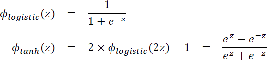
The advantage of the hyperbolic tangent over the logistic function is that it has a broader output spectrum ranging in the open interval (–1, 1), which can improve the convergence of the back-propagation algorithm (Neural Networks for Pattern Recognition, C. M. Bishop, Oxford University Press, pages: 500-501, 1995).
In contrast, the logistic function returns an output signal ranging in the open interval (0, 1). For a simple comparison of the logistic function and the hyperbolic tangent,
let's plot the two sigmoidal functions:
import matplotlib.pyplot as plt
%matplotlib inline

def tanh(z):
    e_p = np.exp(z)
    e_m = np.exp(-z)
    return (e_p-e_m)/(e_p+e_m)

z = np.arange(-5, 5, 0.005)
log_act = logistic(z)
tanh_act = tanh(z)

plt.ylim([-1.5, 1.5])
plt.xlabel('Net input $z$')
plt.ylabel('Activation $\phi(z)$')

plt.axhline(1, color='black', linestyle=':')
plt.axhline(0.5, color='black', linestyle=':')
plt.axhline(0, color='black', linestyle=':')
plt.axhline(-0.5, color='black', linestyle=':')
plt.axhline(-1, color='black', linestyle=':')

plt.plot(z, tanh_act, linewidth=3, linestyle='--', label='Tanh', color='blue')
plt.plot(z, log_act, linewidth=3, label='Logistic', color='green')
plt.legend(loc='lower right')
plt.tight_layout()

plt.show()
As you can see, the shapes of the two sigmoidal curves look very similar; however, the tanh function has double the output space of the logistic function:
Note that we previously implemented the logistic and tanh functions verbosely for the purpose of illustration. In practice, we can use NumPy's tanh function.
Alternatively, when building an NN model, we can use tf.keras.activations.tanh() in TensorFlow to achieve the same results:
np.tanh(z)![]()
tf.keras.activations.tanh(z)![]()
In addition, the logistic function is available in SciPy's special module:
# def logistic(z):
#     return 1.0 / (1.0+np.exp(-z))
# log_act = logistic(z)
log_act![]()
from scipy.special import expit

expit(z)![]()
Similarly, we can use the tf.keras.activations.sigmoid() (note, input value should be tf.float16, tf.float32, tf.float64)function in TensorFlow to do the same computation, as follows:
#z = np.arange(-5, 5, 0.005)
tf.keras.activations.sigmoid(z) 
Rectified linear unit activation
Rectified linear unit (ReLU :11_Training Deep Neural Networks_VarianceScaling_leaky relu_PReLU_SELU _Batch Normalization_Reusing https://blog.csdn.net/Linli522362242/article/details/106935910) is another activation function that is often used in deep NNs. Before we delve into ReLU, we should step back and understand the vanishing gradient problem of tanh and logistic activations.
To understand this problem, let's assume that we initially have the net input ![]() = 20, which changes to
= 20, which changes to ![]() = 25 . Computing the tanh activation, we get 𝜙(
= 25 . Computing the tanh activation, we get 𝜙(![]() ) = 1.0 and
) = 1.0 and
𝜙(![]() ) = 1.0 , which shows no change in the output (due to the asymptotic渐近的 behavior of the tanh function and numerical errors).
) = 1.0 , which shows no change in the output (due to the asymptotic渐近的 behavior of the tanh function and numerical errors).
# def tanh(z):
#     e_p = np.exp(z)
#     e_m = np.exp(-z)
#     return (e_p-e_m)/(e_p+e_m)
# np.tanh(20) ==> 1.0
# np.tanh(25) ==> 1.0

np.tanh(20)![]()
tf.keras.activations.tanh([20, 25])
... ...
tf.keras.activations.tanh() (note, input value should be tf.float16, tf.float32, tf.float64)
# tf.keras.activations.tanh(20.) ==> <tf.Tensor: shape=(), dtype=float32, numpy=1.0>
# tf.keras.activations.tanh(25.) ==> <tf.Tensor: shape=(), dtype=float32, numpy=1.0>
tf.keras.activations.tanh([20., 25.])![]()
This means that the derivative of activations with respect to the net input diminishes[dɪˈmɪnɪʃ](使)减小,减弱; 贬低 as z becomes large. As a result, learning weights during the training phase becomes very slow because the gradient terms may be very close to zero(e.g.![]() ). ReLU activation addresses this issue. Mathematically, ReLU is defined as follows:
). ReLU activation addresses this issue. Mathematically, ReLU is defined as follows:![]()
ReLU is still a nonlinear function that is good for learning complex functions with NNs. Besides this, the derivative of ReLU, with respect to its input, is always 1 for positive input values. Therefore, it solves the problem of vanishing gradients, making it suitable for deep NNs. In TensorFlow, we can apply the ReLU activation as follows:
tf.keras.activations.relu(z)![]()
Now that we know more about the different activation functions that are commonly used in artificial NNs, let's conclude this section with an overview of the different activation functions that we will encounter: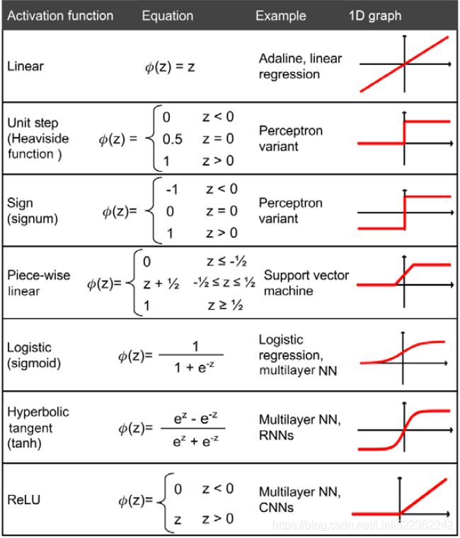
You can find the list of all activation functions available in the Keras API at https://www.tensorflow.org/api_docs/python/tf/keras/activations.
Summary
In this chapter, you learned how to use TensorFlow, an open source library for numerical computations, with a special focus on deep learning. While TensorFlow is more inconvenient to use than NumPy, due to its additional complexity to support GPUs, it allows us to define and train large, multilayer NNs very efficiently.
Also, you learned about using the TensorFlow Keras API to build complex machine learning and NN models and run them efficiently. We explored model building in TensorFlow by defining a model from scratch via subclassing the tf.keras.Model class. Implementing models can be tedious when we have to program at the level of matrix-vector multiplications and define every detail of each operation. However, the advantage is that this allows us, as developers, to combine such basic operations and build more complex models. We then explored tf.keras.layers, which makes building NN models a lot easier than implementing them from scratch.
Finally, you learned about different activation functions and understood their behaviors and applications. Specifically, in this chapter, we covered tanh, softmax, and ReLU.


 7636
7636


 被折叠的 条评论
为什么被折叠?
被折叠的 条评论
为什么被折叠?
 到【灌水乐园】发言


