09_Up and Running with TensorFlow_2_Autodiff_momentum optimizer_Mini-batchGradientDescent_SavingMode

09_Up and Running with TensorFlow_Anaconda3-4.2.0_No module named joblib_KeyError 0_Normal Equation
https://blog.csdn.net/Linli522362242/article/details/106214525

Implementing Gradient Descent

     Let's try using Batch Gradient Descent (introduced in https://blog.csdn.net/Linli522362242/article/details/104005906 Chapter 4) instead of the Normal Equation. First we will do this by manually computing the gradients, then we will use TensorFlow's autodiff feature to let TensorFlow compute the gradients automatically, and finally we will use a couple of TensorFlow's out-of-the-box optimizers.

###############################
WARNING
     When using Gradient Descent, remember that it is important to first normalize the input feature vectors, or else training may be much slower. You can do this using TensorFlow, NumPy, Scikit-Learn's StandardScaler, or any other solution you prefer. The following code assumes that this normalization has already been done.
###############################

     Gradient Descent requires scaling the feature vectors first. We could do this using TF, but let's just use Scikit-Learn for now.

from sklearn.preprocessing import StandardScaler

scaler = StandardScaler()
scaled_housing_data = scaler.fit_transform( housing.data )
scaled_housing_data_plus_bias = np.c_[ np.ones((m,1)), scaled_housing_data ]

print( "mean on row: ", scaled_housing_data_plus_bias.mean( axis=0 ) )
print( "mean on column: ", scaled_housing_data_plus_bias.mean( axis=1 ) )
print( "mean on all: ", scaled_housing_data_plus_bias.mean() )
print( "dataset's shape: ", scaled_housing_data_plus_bias.shape )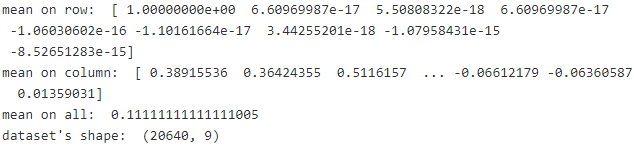

###############################################
https://blog.csdn.net/Linli522362242/article/details/104005906

Note:cost function 

Equation 4-5. Partial derivatives of the cost function(start with  or i >=1)
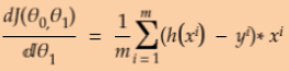== * 2 (without adding the term to the calculation process.)

Equation 4-6. Gradient vector of the cost function ( for equation 4-5)
 Note: == *2

 (without adding the term to the calculation process.)

Equation 4-7. Gradient Descent step 

###############################################

Manually Computing the Gradients
https://docs.w3cub.com/tensorflow~python/tf/constant/

https://www.w3cschool.cn/tensorflow_python/tensorflow_python-jabh2d30.html

The following code should be fairly self-explanatory, except for a few new elements:

• The random_uniform() function creates a node in the graph that will generate a tensor containing random values, given its shape and value range, much like NumPy's rand() function.
   
• The assign() function creates a node that will assign a new value to a variable.
  In this case, it implements the Batch Gradient Descent step .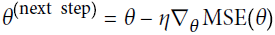
   
• The main loop executes the training step over and over again (n_epochs times), and every 100 iterations it prints out the current Mean Squared Error (mse). You should see the MSE go down at every iteration.

Implementing Gradient Descent

     Gradient Descent requires scaling the feature vectors first. We could do this using TF, but let's just use Scikit-Learn for now.###

n_epochs = 1000
learning_rate = 0.01
                 # "value": a constant value, or a list of values of type "dtype"
X = tf.constant( value=scaled_housing_data_plus_bias, dtype=tf.float32, name="X" )
y = tf.constant( housing.target.reshape(-1,1), dtype=tf.float32, name="y" )
theta = tf.Variable( tf.random_uniform(shape=[ housing.data.shape[1]+1, 1 ], #+since the bias item
                                       minval=-1.0, 
                                       maxval=1.0, 
                                       seed=42
                                      ), 
                    name="theta")
y_pred = tf.matmul(X, theta, name="prediction") # X.dot(theta)
error = y_pred - y
mse = tf.reduce_mean( tf.square(error), name="mse" )
gradients = 2.0/m * tf.matmul( tf.transpose(X), error )############
            #The assign() function creates a node that will assign a new value to a variable.
training_op = tf.assign( theta, theta- learning_rate*gradients )############

init = tf.global_variables_initializer()

with tf.Session() as sess:
    sess.run( init )
    
    for epoch in range(n_epochs):
        if epoch % 100 ==0:
            print("Epoch", epoch, "MSE=", mse.eval() )
        sess.run(training_op)
        
    best_theta = theta.eval()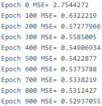

best_theta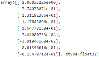

Using autodiff

     The preceding code works fine, but it requires mathematically deriving the gradients from the cost
function (MSE). In the case of Linear Regression, it is reasonably easy, but if you had to do this with deep
neural networks you would get quite a headache: it would be tedious and error-prone易错的. You could use
symbolic differentiation to automatically find the equations for the partial derivatives for you, but the
resulting code would not necessarily be very efficient.

     To understand why, consider the function f(x)= exp(exp(exp(x))). If you know calculus, you can figure out its derivative f′(x) = exp(x) × exp(exp(x)) × exp(exp(exp(x))). If you code f(x) and f′(x) separately and exactly as they appear, your code will not be as efficient as it could be. A more efficient solution would be to write a function that first computes exp(x), then exp(exp(x)), then exp(exp(exp(x))), and returns all three. This gives you f(x) directly (the third term), and if you need the derivative you can just multiply all three terms and you are done. With the naïve approach you would have had to call the exp function nine times to compute both f(x) and f′(x). With this approach you just need to call it three times.

     It gets worse when your function is defined by some arbitrary code. Can you find the equation (or the code) to compute the partial derivatives of the following function?
Hint: don't even try.
Let's compute the function at a=0.2a=0.2 and b=0.3

def my_func(a,b):
    z = 0
    for i in range(100):
        z=a*np.cos(z+i) + z*np.sin(b-i)
    return z

my_func(0.2, 0.3)

     Fortunately, TensorFlow's autodiff feature comes to the rescue: it can automatically and efficiently compute the gradients for you. Simply replace the gradients = ... line in the Gradient Descent code in the previous section with the following line, and the code will continue to work just fine:

Same as above except for the gradients = ... line: 

tf.reset_default_graph()

n_epochs = 1000
learning_rate = 0.01
                 # "value": a constant value, or a list of values of type "dtype"
X = tf.constant( value=scaled_housing_data_plus_bias, dtype=tf.float32, name="X" )
y = tf.constant( housing.target.reshape(-1,1), dtype=tf.float32, name="y" )
theta = tf.Variable( tf.random_uniform(shape=[ housing.data.shape[1]+1, 1 ], #+since the bias item
                                       minval=-1.0, 
                                       maxval=1.0, 
                                       seed=42
                                      ), 
                    name="theta")
y_pred = tf.matmul(X, theta, name="prediction") # X.dot(theta)
error = y_pred - y
mse = tf.reduce_mean( tf.square(error), name="mse" )

###--the gradients(mse, theta)--> 
if return a gradient list [grad1, grad2, grad3], ys=[y1, y2],  xs=[x1, x2, x3], 

tf.gradients(xs, ys):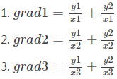  

gradients =  tf.gradients(mse, [theta])[0]

    The gradients() function takes an op (in this case mse) and a list of variables (in this case just theta),
and it creates a list of ops (one per variable) to compute the gradients of the op with regards to each
variable. So the gradients node will compute the gradient vector of the MSE with regards to theta.

training_op = tf.assign( theta, theta- learning_rate*gradients )############

init = tf.global_variables_initializer()

with tf.Session() as sess:
    sess.run( init )
    
    for epoch in range(n_epochs):
        if epoch % 100 ==0:
            print("Epoch", epoch, "MSE=", mse.eval() )
        sess.run(training_op)
        
    best_theta = theta.eval()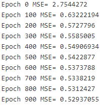

     There are four main approaches to computing gradients automatically. They are summarized in Table 9-2. TensorFlow uses reverse-mode autodiff, which is perfect (efficient and accurate) when there are many inputs and few outputs, as is often the case in neural networks. It computes all the partial derivatives of the outputs with regards to all the inputs in just + 1 graph traversals.

Table 9-2. Main solutions to compute gradients automatically

     Let's compute the function at a=0.2a=0.2 and b=0.3b=0.3, and the partial derivatives at that point with regards to aa and with regards to bb:

tf.reset_default_graph()

a = tf.Variable(0.2, name="a")
b = tf.Variable(0.3, name="b")
z = tf.constant(0.0, name="z0")
for i in range(100):
    z = a*tf.cos(z+i) + z*tf.sin(b-i)
    
grads = tf.gradients(z, [a,b])
init = tf.global_variables_initializer()

with tf.Session() as sess:
    init.run()
    print(z.eval())
    print(sess.run(grads))

##########################################

Autodiff

     This explains how TensorFlow's autodiff feature works, and how it compares to other solutions. Suppose you define a function f(x,y) = , and you need its partial derivatives  and , typically to perform Gradient Descent (or some other optimization algorithm). Your main options are manual differentiation, symbolic differentiation符号微分法, numerical differentiation, forward-mode autodiff, and finally reverse-mode autodiff. TensorFlow implements this last option. Let's go through each of these options.

Manual Differentiation

     The first approach is to pick up a pencil and a piece of paper and use your calculus knowledge to derive the partial derivatives manually. For the function f(x,y) just defined, it is not too hard; you just need to use five rules:

• The derivative of a constant is 0.
• The derivative of λx is λ (where λ is a constant).
• The derivative of is , so the derivative of  is 2x.
• The derivative of a sum of functions is the sum of these functions' derivatives.
• The derivative of λ times a function is λ times its derivative.

From these rules, you can derive Equation D-1:

Equation D-1. Partial derivatives of f(x,y)= 

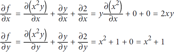
     This approach can become very tedious for more complex functions, and you run the risk of making mistakes. The good news is that deriving the mathematical equations for the partial derivatives like we just did can be automated, through a process called symbolic differentiation.

Symbolic Differentiation符号积分

     Figure D-1 shows how symbolic differentiation works on an even simpler function, g(x,y) = 5 + xy. The graph for that function is represented on the left. After symbolic differentiation, we get the graph on the right, which represents the partial derivative = 0 + 0 × x + y × 1 = y (we could similarly obtain the partial derivative with regards to y).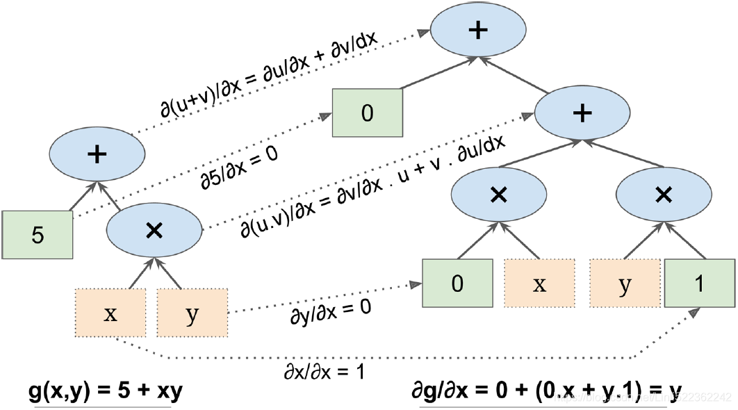

Figure D-1. Symbolic differentiation

     The algorithm starts by getting the partial derivative of the leaf nodes. The constant node (5) returns the constant 0, since the derivative of a constant is always 0. The variable x returns the constant 1 since ∂x/∂x = 1, and the variable y returns the constant 0 since ∂y/∂x = 0 (if we were looking for the partial derivative with regards to y, it would be the reverse( The variable y returns the constant 1 since ∂y/∂y = 1, and the variable x returns the constant 0 since ∂x/∂y = 0 ).

     Now we have all we need to move up the graph to the multiplication node in function g. Calculus tells us that the derivative of the product of two functions u and v is  = ∂v/∂x × u + ∂u/∂x × v. We can therefore construct a large part of the graph on the right, representing 0 × x + y × 1.

     Finally, we can go up to the addition node in function g. As mentioned, the derivative of a sum of functions is the sum of these functions' derivatives. So we just need to create an addition node and connect it to the parts of the graph we have already computed. We get the correct partial derivative: = 0 + ( 0 × x + y × 1) .

     However, it can be simplified (a lot). A few trivial不重要的 pruning steps can be applied to this graph to get rid of all unnecessary operations, and we get a much smaller graph with just one node: ∂g/∂x = y.

     In this case, simplification is fairly easy, but for a more complex function, symbolic differentiation can produce a huge graph that may be tough to simplify and lead to suboptimal performance. Most importantly, symbolic differentiation cannot deal with functions defined with arbitrary code—for example, the following function discussed
in following:

def my_func(a, b):
    z = 0
    for i in range(100):
    z = a * np.cos(z + i) + z * np.sin(b - i)
return z

Numerical Differentiation数值积分

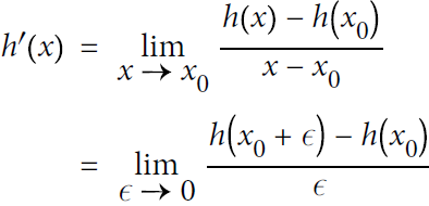
     The simplest solution is to compute an approximation of the derivatives, numerically. Recall that the derivative h′() of a function h(x) at a point is the slope of the function at that point, or more precisely Equation D-2.

Equation D-2. Derivative of a function h(x) at point

     So if we want to calculate the partial derivative of f(x,y) with regards to x, at x = 3 and y = 4, we can simply compute f(3 + ϵ, 4) – f(3, 4) and divide the result by ϵ, using a very small value for ϵ. That's exactly what the following code does:

def f(x,y):
    return x**2*y + y+2

def derivative(f, x, y, x_eps, y_eps):
    return ( f(x+x_eps, y+y_eps) - f(x,y) ) / (x_eps + y_eps)

df_dx = derivative(f, 3, 4, 0.00001, 0)
df_dy = derivative(f, 3, 4, 0, 0.00001)

print(df_dx)
print(df_dy)

     Unfortunately, the result is imprecise (and it gets worse for more complex functions). The correct results are respectively 24 and 10, but instead we get: 

 
     Notice that to compute both partial derivatives, we have to call f() at least three times (we called it four times in the preceding code, but it could be optimized). If there were 1,000 parameters, we would need to call f() at least 1,001 times. When you are dealing with large neural networks, this makes numerical differentiation way too inefficient.

     However, numerical differentiation is so simple to implement that it is a great tool to check that the other methods are implemented correctly. For example, if it disagrees with your manually derived function, then your function probably contains a mistake.

Forward-Mode Autodiff前向自动积分

     Forward-mode autodiff is neither numerical differentiation nor symbolic differentiation, but in some ways it is their love child. It relies on dual numbers对偶数, which are (weird but fascinating) numbers of the form a + bϵ where a and b are real numbers and ϵ is an infinitesimal [ˌɪnfɪnɪˈtesɪml]无限小地 number such that = 0 (but ϵ ≠ 0). You can think of the dual number 42 + 24ϵ as something akin相似的 to 42.0000⋯000024 with an infinite number of 0s (but of course this is simplified just to give you some idea of what dual numbers are). A dual number is represented in memory as a pair of floats. For example, 42 + 24ϵ is represented by the pair (42.0, 24.0).

     Dual numbers can be added, multiplied, and so on, as shown in Equation D-3.
Equation D-3. A few operations with dual numbers

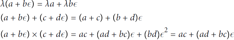  (since = 0 )

     Most importantly, it can be shown that h(a + bϵ) = h(a) + b × h′(a)ϵ, so computing h(a + ϵ) gives you both h(a) and the derivative h′(a) in just one shot. Figure D-2 shows how forward-mode autodiff computes the partial derivative of f(x,y)=with regards to x at x = 3 and y = 4. All we need to do is compute f(3 + ϵ, 4); this will output a dual number whose first component is equal to f(3, 4) and whose second component is equal to .
 Figure D-2. Forward-mode autodiff

     To compute  =10 we would have to go through the graph again, but this time with x = 3 and y = 4 + ϵ.

     So forward-mode autodiff is much more accurate than numerical differentiation, but it suffers from the same major flaw缺点: if there were 1,000 parameters, it would require 1,000 passes through the graph to compute all the partial derivatives. This is where reverse-mode autodiff shines: it can compute all of them in just two passes through
the graph.

Reverse-Mode Autodiff

     Reverse-mode autodiff is the solution implemented by TensorFlow.

• It first goes through the graph in the forward direction (i.e., from the inputs to the output) to compute the value of each node.
   
• Then it does a second pass, this time in the reverse direction (i.e., from the output to the inputs) to compute all the partial derivatives.

 Figure D-3. Reverse-mode autodiff

     Figure D-3 represents the second pass. During the first pass, all the node values were computed, starting from x = 3 and y = 4. You can see those values at the bottom right of each node (e.g., :  x × x =3 × 3= 9,
× y = 9 × 4 = 36, y + 2 = 4 + 2 = 6,  36 + 6 = 42 ). The nodes are labeled n1 to n7 for clarity. The output node is : f(3,4) = = 42.

     The idea is to gradually go down the graph, computing the partial derivative of f(x,y) with regards to each consecutive node, until we reach the variable nodes. For this, reverse-mode autodiff relies heavily on the chain rule, shown in Equation D-4.

Equation D-4. Chain rule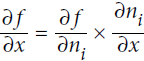  
Since is the output node, f = so trivially = 1.

     Let's continue down the graph to : how much does f vary when varies? The answer is . We already know that = 1, so all we need is . Since simply performs the sum =, we find that , so   .

     Now we can proceed to node : how much does f vary when varies? The answer is . Since , we find that , so .

     The process continues until we reach the bottom of the graph. At that point we will have calculated all the partial derivatives of f(x,y) at the point x = 3 and y = 4. In this example, we find ∂f/∂x =  and ∂f/∂y = . Sounds about right!

     Reverse-mode autodiff is a very powerful and accurate technique, especially when there are many inputs and few outputs, since it requires only one forward pass plus one reverse pass per output to compute all the partial derivatives for all outputs with regards to all the inputs. Most importantly, it can deal with functions defined by arbitrary code. It can also handle functions that are not entirely differentiable, as long as you ask it to compute the partial derivatives at points that are differentiable.
###############################
     If you implement a new type of operation in TensorFlow and you want to make it compatible with autodiff, then you need to provide a function that builds a subgraph to compute its partial derivatives with regards to its inputs. For example, suppose you implement a function that computes the square of its input . In that case you would need to provide the corresponding derivative function f′(x) = 2x. Note that this function does not compute a numerical
result, but instead builds a subgraph that will (later) compute the result. This is very useful because it means that you can compute gradients of gradients (to compute second-order derivatives, or even higher-order derivatives).

##########################################

How could you find the partial derivatives of the following function with regards to a and b?

Using an Optimizer

     So TensorFlow computes the gradients for you. But it gets even easier: it also provides a number of optimizers out of the box, including a Gradient Descent optimizer. You can simply replace the preceding gradients = ... and training_op = ... lines with the following code, and once again everything will just work fine:

tf.reset_default_graph()

n_epochs = 1000

X = tf.constant(scaled_housing_data_plus_bias, dtype=tf.float32, name="X")
y = tf.constant(housing.target.reshape(-1,1), dtype=tf.float32, name="y")
theta = tf.Variable(tf.random_uniform([n+1,1], -1.0, 1.0, seed=42), name="theta")
y_pred = tf.matmul(X, theta, name="predictions")
error = y_pred - y
mse = tf.reduce_mean( tf.square(error), name="mse" )

cost function   VS previously, Gradient Descent step 

# gradients =  tf.gradients(mse, [theta])[0]
# training_op = tf.assign( theta, theta- learning_rate*gradients )
learning_rate = 0.01########
optimizer = tf.train.GradientDescentOptimizer(learning_rate=learning_rate)
training_op = optimizer.minimize(mse)

init = tf.global_variables_initializer()

with tf.Session() as sess:
    sess.run(init)
    
    for epoch in range(n_epochs):
        if epoch % 100 ==0:
            print( "Epoch", epoch, "MSE = ", mse.eval() )
        sess.run( training_op)
    best_theta = theta.eval()
    
print("\nBest theta:\n", best_theta)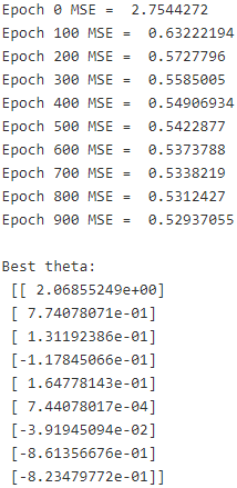

     If you want to use a different type of optimizer, you just need to change one line. For example, you can use a momentum [moʊˈmentəm]动力  optimizer (which often converges much faster than Gradient Descent; see Chapter 11) by defining the optimizer like this:

Using a momentum optimizer

tf.reset_default_graph()

n_epochs = 1000
learning_rate = 0.01

X = tf.constant( scaled_housing_data_plus_bias, dtype=tf.float32, name="X" )
y = tf.constant( housing.target.reshape(-1, 1), dtype=tf.float32, name="y" )
theta = tf.Variable( tf.random_uniform([n+1, 1], -1.0, 1.0, seed=42), name="theta" )
y_pred = tf.matmul( X, theta, name="predictions" )
error = y_pred - y
mse = tf.reduce_mean( tf.square(error), name="mse" )

optimizer = tf.train.MomentumOptimizer( learning_rate=learning_rate, momentum=0.9 )
training_op = optimizer.minimize(mse)

init = tf.global_variables_initializer()

with tf.Session() as sess:
    sess.run(init)
    
    for epoch in range(n_epochs):
        sess.run( training_op )
        
    best_theta = theta.eval()
    
print("Best theta:\n", best_theta)

Feeding Data to the Training Algorithm

     Let's try to modify the previous code to implement Mini-batch Gradient Descent. For this, we need a way to replace X and y at every iteration with the next mini-batch. The simplest way to do this is to use placeholder nodes. These nodes are special because they don't actually perform any computation, they just output the data you tell them to output at runtime. They are typically used to pass the training data to TensorFlow during training. If you don't specify a value at runtime for a placeholder, you get an exception.

     To create a placeholder node, you must call the placeholder() function and specify the output tensor's data type. Optionally, you can also specify its shape, if you want to enforce it. If you specify None for a dimension, it means "any size." 
     For example, the following code creates a placeholder node A, and also a node B = A + 5. When we evaluate B, we pass a feed_dict to the eval() method that specifies the value of A. Note that A must have rank 2 (i.e., it must be two-dimensional) and there must be three columns (or else an exception is raised), but it can have any number of rows.

Placeholder nodes

tf.reset_default_graph()

A = tf.placeholder( tf.float32, shape=(None, 3) )
B = A + 5
with tf.Session() as sess:
    B_val_1 = B.eval( feed_dict={A: [[1,2,3]]
                                }
                    )
    B_val_2 = B.eval( feed_dict={A: [[4,5,6],
                                     [7,8,9]
                                    ]
                                }
                    )

print(B_val_1)

print(B_val_2)

##############################

Note
     You can actually feed the output of any operations, not just placeholders. In this case TensorFlow does not try to evaluate these operations; it uses the values you feed it.
##############################

     To implement Mini-batch Gradient Descent, we only need to tweak the existing code slightly. First change the definition of X and y in the construction phase to make them placeholder nodes:

n_epochs = 1000
learning_rate = 0.01


tf.reset_default_graph()

X = tf.placeholder( tf.float32, shape=(None, n+1), name="X" ) ######
y = tf.placeholder( tf.float32, shape=(None, 1), name="y" )   ######

theta = tf.Variable( tf.random_uniform([n+1, 1], -1.0, 1.0, seed=42), name="theta" )
y_pred = tf.matmul( X, theta, name="prediction" )
error = y_pred - y
mse = tf.reduce_mean( tf.square(error), name="mse" )

optimizer = tf.train.GradientDescentOptimizer( learning_rate = learning_rate )
training_op = optimizer.minimize(mse)

init = tf.global_variables_initializer()
n_epochs = 10

Then define the batch size and compute the total number of batches:

batch_size = 100
n_batches = int(np.ceil( housing.data.shape[0]/batch_size )) #housing.data.shape[0]: the number of samples

      Finally, in the execution phase, fetch the mini-batches one by one, then provide the value of X and y via the feed_dict parameter when evaluating a node that depends on either of them.

def fetch_batch( epoch, batch_index, batch_size ):
    np.random.seed( epoch*n_batches + batch_index )
    indices = np.random.randint(m,size=batch_size)
    X_batch = scaled_housing_data_plus_bias[indices]
    y_batch = housing.target.reshape(-1,1) [indices]
    return X_batch, y_batch

with tf.Session() as sess:
    sess.run(init)
    
    for epoch in range(n_epochs):
        for batch_index in range(n_batches):
            X_batch, y_batch = fetch_batch( epoch, batch_index, batch_size )
            sess.run( training_op, feed_dict={X: X_batch, y: y_batch})
            
    best_theta = theta.eval()


best_theta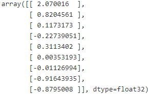

############################
NOTE
     We don't need to pass the value of X and y when evaluating theta since it does not depend on either of them.


############################

Saving and Restoring Models

     Once you have trained your model, you should save its parameters to disk so you can come back to it whenever you want, use it in another program, compare it to other models, and so on. Moreover, you probably want to save checkpoints at regular intervals during training so that if your computer crashes during training you can continue from the last checkpoint rather than start over from scratch.

     TensorFlow makes saving and restoring a model very easy. Just create a Saver node at the end of the construction phase (after all variable nodes are created); then, in the execution phase, just call its save() method whenever you want to save the model, passing it the session and path of the checkpoint file:

tf.reset_default_graph()

n_epochs = 1000
learning_rate = 0.01

X = tf.constant( scaled_housing_data_plus_bias, dtype=tf.float32, name="X" ) # X node
y = tf.constant( housing.target.reshape(-1,1), dtype=tf.float32, name="y" )  # y node
theta = tf.Variable( tf.random_uniform([n+1, 1], -1.0, 1.0, seed=42 ), name="theta" ) # theta node
y_pred = tf.matmul(X, theta, name="predictions")                             # predictions node
error = y_pred-y                                                             #sub node
                     # Square node   #for (y_pred-y)**2 (Const int 2 node)
mse = tf.reduce_mean( tf.square(error), name="mse" )                        # mse node
#GradientDescent: Next theta=current theta - learning_rate * gradients
optimizer = tf.train.GradientDescentOptimizer( learning_rate=learning_rate ) # GradientDescent node
training_op = optimizer.minimize(mse) # gradients node: 2/m * X^T * (y_pred - y) 
init = tf.global_variables_initializer()                                    #init node
# Just create a Saver node at the end of the construction phase (after all "variable nodes" are created)
saver = tf.train.Saver() ###############Saver##############                #save node

with tf.Session() as sess:
    sess.run(init)
    
    for epoch in range(n_epochs):
        if epoch%100 ==0: # checkpoint every 100 epochs
            print( "Epoch", epoch, "MSE=", mse.eval() )
            save_path = saver.save(sess, "/tmp/my_model.ckpt") #passing it the session and path of the checkpoint file:
        sess.run(training_op)
        
    best_theta = theta.eval()
    save_path = saver.save(sess, "/tmp/my_model_final.ckpt")

 # output the best(minimum of ) mse in every 100 epoch

best_theta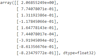

     Restoring a model is just as easy: you create a Saver at the end of the construction phase just like before, but then at the beginning of the execution phase, instead of initializing the variables using the init node, you call the restore() method of the Saver object:

with tf.Session() as sess:
    saver.restore(sess, "/tmp/my_model_final.ckpt")
    best_theta_restored = theta.eval()

np.allclose(best_theta, best_theta_restored)

     By default a Saver saves and restores all variables under their own name, but if you need more control, you can specify which variables to save or restore, and what names to use. For example, the following Saver will save or restore only the theta variable under the name "weights":

# If you want to have a saver that loads and restores theta with a different name, such as "weights":
saver = tf.train.Saver({"weights": theta})

     By default the saver also saves the graph structure itself in a second file with the extension .meta. You can use the function tf.train.import_meta_graph() to restore the graph structure. This function loads the graph into the default graph and returns a Saver that can then be used to restore the graph state (i.e., the variable values):

tf.reset_default_graph()

# notice that we start with an empty graph.
saver = tf.train.import_meta_graph("/tmp/my_model_final.ckpt.meta") #this loads the graph structure
theta = tf.get_default_graph().get_tensor_by_name("theta:0")
#Tensor("theta:0", shape=(9, 1), dtype=float32_ref)

with tf.Session() as sess:
    saver.restore(sess, "/tmp/my_model_final.ckpt") # this restores the graph's state
    best_theta_restored = theta.eval() #not shown in the book

np.allclose(best_theta, best_theta_restored)

This means that you can import a pretrained model without having to have the corresponding Python code to build the graph. This is very handy when you keep tweaking and saving your model: you can load a previously saved model without having to search for the version of the code that built it.

https://www.tensorflow.org/api_docs/python/tf/Graph

Visualizing the Graph and Training Curves Using TensorBoard

https://blog.csdn.net/Linli522362242/article/details/106325257